KEYWORDS: evolution computation technologies, genetic algorithms, differential evolution, high-dimensional optimization problems
DIRECTLY TO DOWNLOAD: here

NOTE: This page has nothing to do with Marquis de Sade. To gather some information about this topic, follow for example this link:

Recent times optimization methods, especially evolution computational technologies, belong to the mostly discussed topics. Genetic algorithms, relatively new approach in this area (their development has begun about ten or fifteen years ago), are becoming to be more and more popular tools for solving growing spectrum of optimization tasks and some practical applications are already known.

We have started to deal with these methods in summer 2000. There was a need for equally reliable, effective and versatile algorithm that could help us to solve a relatively disparate set of optimization problems that nowadays come to focus. Except others the following problems have been investigating:

1. identification of material model parameters,
2. regression analysis,
3. training of a neural network that can be used to approximate estimation of material model parameters from experimental results
4. topological optimizations
5. some engineering tasks, such as optimization of reinforced concrete beams and other structures and structural elements.

There are some tasks with a relatively large number of unknowns among mentioned above. Optimization of reinforced concrete beam has between 18 and 21 unknown parameters; neural network that is going to identify material model parameters may have up to 200 unknown (these are so called synaptic weights - their values are the result of neural network training). Naturally, with the growth of dimension the time consumption of any possible optimization method also grows. Finding a method for which this increase is as low as possible (that means not worse that linear) was one of our most important aims in the first phase of our research.

Difficulties on local extremes

Emergency of a fall to a local extreme is a next painful difficulty of genetic algorithms, as long as of any other optimization method. Generally, there are two antagonistic ways to solve this problem. The first one that has beeing used for example by M.Lep? in his work [#!Matej!#] consist in some kind of a convergence retardation. This should ensure that the algorithm will not decide to pop in a first - and thus probably local - extreme that comes it's way too soon. This method is usually called simulated anealing; in our opinion is usable successfully in cases where many local extremes are situated not far from each other and their values do not dramatically differ. Good idea of a function with this feature can give a concept "warted hill".

Another way to deal with local extreme comes out from Monte Carlo method. We suppose that to find the global extreme among large amount of local ones it is necessary to repeat the computation many times starting from different initial states. This way can ensure good chance to find right solution even in verycomplicated cases, but it is still possible to introduce minimally two reasons against. At first, an algorithm can repeat a computation many times with the same results which is going to increase the time consumption. The second, let's try to imagine such a case: graph of an optimized function has a character of vast mountains with sheer sides but still not very high, and global extreme is somewhere beside it on a narrow peak; another idea could be a mosque with several minarets. In this case algorithm will end in some of the tops of our mountain massive everytime, no matter what the initial state was; the right solution will not be found ever or only with very small probability.

We suppose that ideal universal strategy should be able to find out any (let's say acceptable) solution as quickly as possible, store it and proceed to find another, maybe better one. Practical points of view also support this opinion: if our problem is very complicated, this strategy gives us much better chance to acquire at least some usable solution. So, within the first phase of our research we have fixed to find a method, as effective but (meanwhile) as simple and as transparent as possible, that it is going to be able solve quickly and reliably some simple case, no matter how large the amount of unknowns is.

As it has come in sight, some of the large set of the methods we have tested are able to resolve not very difficult cases of local extremes relatively well. Still we decided to deal with this inconvenient question as a stand-alone problem within the next phase of our research which is not a subject of this text.

Real domains

Genetic algorithms themselves (in a manner they were developed) work with binary strings (so called chromosomes). But obviously, all the cases (mentioned above) that are in the focus of our interests are defined on real domains. In the past, there were some propositions how to modify binary genetic algorithm to operate on a real domain, but these techniques bring indispensable problems. For example, it is possible to construct some kind of a maping of the binary strings to real numbers but this technique restrain computation and can also cause negative effect that originaly continuous function gains a non-continuous behaviour: Small change of a binary chromosome can lead to a large change of the mapped floating point number and together a large change of a function value as well. The experience shows that this effect can strongly deteriorate a quality of an algorithm. Choice of a resolution can be another difficult problem itself, like for example for neural network training. These are the reasons that lead us to a searching a method which is able to operate on real numbers straightly and naturally instead of binary chromosomes

First we focused on the most recent type of an optimization method - the differential evolution. Next, with respect to what was said before about our imagination of ideal univerzal optimization strategy we started to develope a method that can reach any (even maybe local) extreme as soon as possible regardless the problem dimension. We have combined ordinal genetic algorithm with Rainer Storn's operators into the SADE technology.

NOTE: SADE means Simplified Atavistic Differential Evolution and has nothing to do with Marquis de Sade.

Algorithm SADE

Although is classical genetic algorithm that operates on binary chromosomes relatively simple and its behaviour is fairly described by so called scheme theorem , impacts of recombinative operators to mapped floating point numbers are much less transparent and imaginable after conversion to real domains. The same could be said for behaviour of operators designed  for the differential evolution.

In our opinion this is relatively serious problem. We consider the transparent and imaginable algorithm to have a lot of advantages from a certain point of view. First of all, many improvements can be proposed by consideration so it is not necessary to proceed by trial and error method, and the lacks of algorithm behaviour together with implementation mistakes can be discovered easily. Also, simple algorithm is easy to realize and if it is well designed there is a pretty good chance that it will be effective and reliable.

Experience shows that when designing an evolution algorithm, it is not necessary to copy processes running in real nature strictly. So we decided to construct our new algorithm to be as simple and as transparent as possible. Technology SADE is a result of this trial. It is a combination technology of common genetic algorithm that uses simplified cross-over operator3 taken from differential evolution instead its original binary form. Next, we have extended this method with mutate and boundary mutate operators, which is going to be described later.

We introduce here this algorithm written in C-language4 in a slightly modified fashion (to improve readability) compared with our original source codes.
The released source code (made by Anicka) that is able to be compiled and tested can be downloaded from here.

void main ( void ) {     int i=0,g=0;     double bsf;     initialize_randoms ();     create_fitness_function ();     compute_radioactivity ();     bsf = FIRST_GENERATION ();     while ( to_continue ( bsf ) )     {         MUTATE ();         BOUNDARY_MUTATE ();         CROSS ();         bsf = EVALUATE_GENERATION ();         SELECT();         i++;         if ( i==50 )         {             i=0;             g++;             printf ( "G=%d bsf=%f top=%f\n", 50*g, bsf, top );         }     }     printf ( "G=%d bsf=%f top=%f\n", 50*g+i, bsf, top );     destroy_all (); }

.
 As usual with evolution technologies, first step is to generate random starting generation (function FIRST_GENERATION). Then we repeat the cycle containing evaluation of actual generation (function EVALUATE_GENERATION) and creating new generation (by calling SELECT, MUTATE, BOUNDARY_MUTATE and CROSS_OVER sequentially) until some stopping criteria (to_be_continued) is full.

Chromosomes themselves will be marked as CH in the following source code specimens, i-th chromosome is then CH[i], length of a chromosome id chlen. Variables SelectedSize, PoolSize and ActualSize have these meanings: during the computational procedure the amount of "living" chromosomes periodically changes. Everytime when new generation is created this amount is equal to PoolSize, function EVALUATE_GENERATION operates on this number of chromosomes. Function SELECT then decreases number of "living" chromosomes to SelectedSize so all genetic operators works with this amount. This way use of a mating pool, a term often mentioned in literature, is not necessary.

We are not going to discuss function to_be_continued in detail here. It concerns the stopping criteria question which can be a stand alone topic and it is described deeply in many well known titles. Let's say only that it works with a variable bsf (means "best so far") which stores the best solution that has been found until actual step.

Now let's suppose that some function new_point that generates random solution vector from a function domain is available. Then function FIRST_GENERATION is trivial and is introduced here only for the reason of perfection.
 

double FIRST_GENERATION ( void) {     int i;     double bsf;     CH = new p_double [PoolSize];     for ( i=0; i<PoolSize; i++ )     {         CH[i] = new_point ();     }     ActualSize = PoolSize;     bsf = EVALUATE_GENERATION ();     SELECT ();     return bsf; }

Function EVALUATE_GENERATION is also very simple. It uses calling of optimized function fitness; value returned by it is then stored into array F and best value of current generation is updated by the way and stored into variable btg (means "best this generation"). Variable start has to ensure that fitness function is called only for chromosomes for which the function value not known and not for chromosomes that survived from the previous generation.
 

double EVALUATE_GENERATION ( void ) {     double btg=0.0;     int i;     static int start=0;     for ( i=start; i<ActualSize; i++ )     {         Force[i] = fitness ( CH[i] );         if ( Force[i]>btg ) btg = Force[i];     }     if ( start==0 ) start = SelectedSize;     return btg; }

Selection

Function SELECT represents the kernel itself of en evolution algorithm itself. Its aim is to provide progressive improvement of the whole population, which is realized by reducing the number of "living" chromosomes together with conservation of better ones. Modified tournament strategy is used for this purpose: two chromosomes are chosen randomly from a population, then they are compared and the worse of them is going to be cast off (it is implemented as enlistment of it to the end of an array and decreasing variable ActualSize by one).
 

void SELECT ( void ) {     double *h;     int i1, i2, dead, last;     while ( ActualSize > SelectedSize )     {         i1 = random_int ( 0,ActualSize );         i2 = random_int ( 1,ActualSize );         if ( i1==i2 ) i2--;         if ( Force[i1] >= Force[i2] ) dead = i2;         else dead = i1;         last = ActualSize-1;         h = CH[last];         CH[last] = CH[dead];         CH[dead] = h;         Force[dead] = Force[last];         ActualSize--;     } }

Tournament kind of selection has many advantages compared to others so it has become to be the most popular selection technology. Let's introduce these reasons:

1. simplicity and low computational complexity; for example to perform roulette selection a demanding computation of so called roulette is necessary,
2. it conserves population diversity thanks to good chance to survive even for badly performing chromosomes; this usually has possitive impact to the quality of the final result,
3. determination to premature convergence decreases. From other point of view, there is a relatively high probability that the best chromosome will not survive to the next generation, which is a big drawback of this method. To prevent this, we choose everytime the one that should not survive so whenever the best chromosome engages a tournament or not, always survives.

Classical mutation operator usually randomly selects one chromosome and alters one of its coordinates (again randomly chosen). Some modifications apply this to more than only to one coordinate them or to all, which means that embedded chromosome is completely replaced by a brand new one. We have implemented mutate operator in that way at the begining and the results were not bad.

Experiments with optimization of a reinforced concrete beam led us to another modification: randomly chosen chromosome is not replaced by a new one but is only moved that direction by some part of their distance. This modification caused significant improvement on most tested functions. Efficiency of this method depends how far the chromosome is moved in fact, which indicate parameter mutation_rate.

Parameter radioactivity determines the number of chromosomes that are going to be mutated each generation. For example, if radioactivity is 1% and number SelectedSize is equal to 100, than single chromosome will be mutated for each generation. As radioactivity is usually low, some problems may rise within small sizes of population. If radioactivity is 1% again and population size is only 20, one chromosome should be mutated each fifth generation. We have resolved this by determination maximum number of chromosomes that can be mutated in a single generation step and reducing mutation probability in corresponding way (in our example mutants is equal to one and reduced_radioactivity is equal to 20 %)
 

void MUTATE ( void ) {     double p, *x;     int i, j, index;     for ( i=0; i<mutants; i++ )     {         p = random_double ( 0,1 );         if ( p<=reduced_radioactivity )         {             index = random_int ( 0,SelectedSize );             x = new_point();             for ( j=0;  j<Dim; j++ )             {                 CH[ActualSize][j] = CH[index][j]+mutation_rate*( x[j]-CH[index][j] );             }             delete [] x;             ActualSize++;         }     } }

Boundary mutation

As mentioned above the diversity of the population should be kept to be at certain minimal level during computation. This brings a negative effect of convergence decceleration which could be oppressive within high problem dimensions. This is why we have introduced boundary mutate operator. Its aim is to grub the near neighbourhood of better chromosomes and so make searching for more and more presious solution faster.

This operator changes all coordinates of chosen chromosome by a random value in given interval which is determined by parameter mutagen. The same considerations as within the mutate operator apply for the probability of boundary mutation.
 

void BOUNDARY_MUTATE ( void ) {     double p,dCH ;     int i,j,index ;     for ( i=0; i<mutants; i++ )     {         p = random_double( 0,1 );         if ( p <= reduced_radioactivity )         {             index = random_int( 0, SelectedSize );             for ( j=0; j<Dim; j++ )             {                 dCH = random_double( -mutagen,mutagen );                 CH[ActualSize][j] = CH[index][j]+dCH;             }             ActualSize++;         }     } }

Crossing over

As radioactivity is usually low operators described above create only a small amount of new chromosomes (typically one or two each generation). The rest up to the number PoolSize fills cross-over operator, based upon sequential scheme: choose randomly two chromosomes, compute their difference vector, multiply it by a coefficient cross_over_rate and add it to the third, also accidentally selected chromosome.
 

void CROSS ( void ) {     int i1,i2,i3,j ;     while ( ActualSize < PoolSize )     {         i1 = random_int( 0,SelectedSize );         i2 = random_int( 1,SelectedSize );         if ( i1==i2 ) i2--;         i3 = random_int( 0,SelectedSize );         for ( j=0 ; j<Dim ; j++ )         {             CH[ActualSize][j] = CH[i3][j]+cross_rate*( CH[i2][j]-CH[i1][j] ) ;         }         ActualSize++;     } }

Figure 1. Geometric meaning of the cross-over operation
 

Although operators used within SADE method are not similar to their opposites known with classical genetic algorithms, we consider SADE to be still a genetic-type method. Our version of the operators is a result of a relatively long development (including even for example introducing boundary-mutate operator). Some idea about the reasonable values of the parametres mentioned above also came as results of this development. Of course they are depending from a general counsel of algoritm: if it has to find any usable extreme as soon as possible or to rise the probability of finding right solution among large number of local extremes. Naturally, these two demands are contradictory.

Still seems that resolving the local extremes problem is too tough task for this simple algorithm yet. So, in our opinion, it is generally better to optimize this method for speed and the local extreme problem solve as a stand-alone chapter.

Let's discuss these parameter one by one at this point.

SelectedSize: number of chromosomes which functions mutate, boundary mutate and cross-over operate on; appears that if the aim is the speed of convergence this value should be set to some lower value such as 10; opposite, if we would like to avoid premature convergence, cover larger space and increase the probability of finding global extrem within more complicated cases, it is necessary to increase this number to , or even more,

PoolSize: maximum number of chromosomes; function SELECT chooses better ones from this amount; usually this number is set two times bigger than SelectedSize,

radiactivity: probability of the mutation and the boundary mutation; the experimental computations show that its optimal value is around 5%; the algorithm itself uses parameters mutants and reduced_radioactivity which are determined using function compute_radioactivity:
 

void compute_radioactivity ( void ) {     double p, rn;     p = radioactivity*( double )SelectedSize;     rn = ceil ( p );     reduced_radioactivity = p/rn;     mutants = ( int )rn; }

mutation_rate: tells how far moves the mutated chromosome to the other that is picked up accidentally from a domain; usually set to 50%,

mutagen: the size of an interval within boundary mutation changes all coordinates of mutated chromosome; to determine its value is a complicated problem; for example, if some variable has its given resolution, it is better to set mutagen equal to it; in other cases it is necessary to try more different values and pick up the one that gives best result,

cross_over_rate: this parameter has probably the most important impact to the algorithm behaviour; it seems that if we want to speed up convergence this parameter should be set to some lower value (like 5 or 10%), opposite, higher values of this parameter could assure better probability to solve the local extreme problem.

SADE method testing: Study of computational complexity with respect to problem dimension

Grow of time consumption (usualy given by number of fitness function calls needed to find global extreme) within problem dimension we consider to be the most important characterization of any evolution technology. Obviously, it depends on the manner of an optimized function.

For the purpose of our experimental computations (let's say benchmark tests) we have chosen certain function which has single extreme on the top of a high and narrow peak (function with this appearance we mark as "type 0"). Here let's introduce its formula:

 In equation above vector stand as a variable and as the point of a global extreme (top of the peak), and are parameters that influence function shape, first of them a height of the peak and the second its width. Figure bellow shows example of such function.

Figure 2: Example of type 0 function

 It is necessary to point out that although this example function has only a single extreme, to find it out with a precision of that was requested by our test conditions is non-trivial task for several reasons. At first, in the very near surround of the extreme itself function is so grasp that even a futile change of the coordinates cause large change of a function value; in such a case it is very difficult for the algorithm to determine which way leads to the top, because even try in the right direction can jump across the top. Next, the peak is very narrow and approves on very small part of a domain; this disproportion increase very quickly with problem dimension. So, chosen function can examine resolution ability of an algoritms hardly. (Ability to adapt its resolution is an interesting advantage of differencial evolution opposite to binary genetic algorithm which resolution is given a priori and cannot be changed.)

Algorithm parameters were set to following values:

SelectedSize=10
PoolSize=20
radioactivity=5%
mutation_rate=50%
mutagen=1.0
cross_over_rate=10%

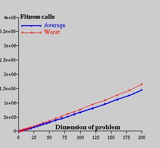
Figure 4: Time consumption with respect to the problem dimension

The convergence process is shown on the sequential graphs. Figure 4 shows the process for the problem dimension 2 and Figure 5 for the problem dimension 50. As could be seen, if the problem dimension is small, algorithm finds the approximate location of the peak very quickly and most of the time spends by improving the solution; opposite, if the problem dimension is bigger, convergence is much more fluent.

Figure 3: Convergence process within the problem dimension 2

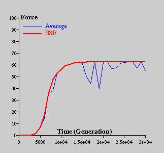
Figure 5: Convergence process within the problem dimension 50

 Let's introduce two more studies of many others performed during our research, that characterize best the behaviour of our algorithm. Influence of the boundary mutation operator appears to be quite interesting. The study was performed with the same conditions as previous one except this operator was completely inactivated. As was pointed out, time consumption of problem solution grows approximately three times regardless the problem dimension. So this operator speeds up a convergence, but has no effect to general behaviour of the method. Some other tests show that the mutate operator absence causes total misfunction of the method on any higher dimension, for example within the problem dimension 50 method cannot climb up more than to about 2% of function maximal value in the same time as the originally configured method finds the final solution.

Next study shows the case, when demanded precision was decreased from 0.001 to 0.5. Within this, time consumption of a method decrease to about one half. This means that algorithm needs the same time to find a peak itself as to find the very sharp final solution. Results of both studies are introduced in picture and a shorten table bellow.

Figure 6: Comparation of results that were reached using boundary mutation or not and with precision lower to 0.5.
 

Problem dimension	Average	Average	Average
1	465	577	196
2	3185	7315	1392
5	17605	47889	7692
10	46956	129635	20817
20	106695	299841	48182
50	304327	858272	134951
100	663084	1844576	303218
200	1446545	3963486	654503
Boundary mutation	On	Off	On
Precision	0.001	0.001	0.5

    Ondra Hrstka email: <ondra@klobouk.fsv.cvut.cz> hmpg: http://klobouk.fsv.cvut.cz/~ondra
    Anicka Kucerova email: <anicka@klobouk.fsv.cvut.cz> hmpg: http://klobouk.fsv.cvut.cz/~anicka
    Matej Leps email: <leps@klobouk.fsv.cvut.cz> hmpg: http://klobouk.fsv.cvut.cz/~leps

Last Update: January 6 2009