1 Introduction

Highway bridges are subjected to experimental analysis of their vibration before they are put into service. The aim of experimental analysis is to determine eigenfrequencies and eigenmodes of the bridges. In order to perform the experiments smoothly and as much precisely as possible, it is useful to determine the eigenfrequencies and eigenmodes by numerical analysis in advance. Sensors should be located in antinodes because of significant displacements which can be measured more precisely than small displacements near the vibration nodes, [?].

The bridges analysed are highway concrete prestressed bridges in Prague. They are six-span structures made from the concrete C35/45-XF2+XD1. The length of the left bridge is 560.976 m (71.999 + 84.248 + 101.905 + 115.170 + 115.153 + 72.501) while the right bridge has the length 551.540 m (72.000 + 83.737 + 99.952 + 112.436 + 112.246 + 71.169). Both bridges are horizontally curved with radius 747.5 m and 753.75 m for the left and right bridge, respectively.

The cross sections of the bridges are changing along the length with respect to the quadratic parabola. The maximum height of the cross section is 6.5 m over the piers while only 3.135 m in the span centers. Each pier is created by four columns with a variable cross section.

2 Finite Element Model

With respect to the complicated bridge geometry, a three-dimensional finite element model was created. The model is based on brick finite elements with eight nodes and linear approximation functions. The three-dimensional model was used because of the curved shape of the bridge. In order to generate the mesh as easily as possible, the bridge was modelled as a straight one and a special short computer code was developed which bends the original mesh into the curved one. Special attention was devoted to the bridge bearings. In order to describe the bearings correctly, local coordinate systems were defined in the nodes of the mesh because of the movable supports.

In the finite element model, the bridge piers were replaced by a set of 588 springs. The bridge piers were modelled separately because they are also curved and even non-prismatic. Each pier was described by its three-dimensional model and all neccessary stiffnesses were obtained. The bridge stiffeners near the bridge supports were also modelled by spring elements.

The mesh contains 51 642 nodes, 39 750 finite brick elements, 588 bar elements representing the bridge piers and stiffeners, 154 926 unknowns (degrees of freedom). The equation of motion of undamped free vibration has the form

M ¨d + Kd = 0 , (1)

where M is the mass matrix, K is the stiffness matrix,

is the vector of nodal accelerations and d is the vector of nodal displacements. The eigenvalue problem is described by the equation

(K − ω20M )v = 0 , (2)

where v is the eigenvector and ω₀ is the natural circular frequency. The eigenfrequencies and eigenvectors were computed by the subspace iteration method which is a generalization of the inverse iteration method. Instead of one vector used in the inverse iteration, the subspace method deals with several vectors simultaneously located in the modal matrix V . Columns of the modal matrix V are orthonormalized in every iteration step and approximations of the eigenvalues are computed in the form

2 T Ω 0 = V KV . (3)

The orthonormalization is based on the Gram-Schmidt method. The subspace iteration is summarized in table 1. More details about the method can be found in references [?] and [?].

Table 1: The subspace iteration method.

definition of initial vectors V ₀, k = 0

iterate k = 0, 1, 2,…

_k+1 = K⁻¹MV _k

_k+1 → V _k+1 : V _k+1^TMV _k+1 = I

Ω_0,k+1 = V _k+1^TKV _k+1

if k > 1 and Ω_0,k+1 − Ω_0,k < εI, break

The system of linear algebraic equations is solved by a sparse direct solver based on the modified minimum degree algorithm which can be found e.g. in reference [?]. The stiffness matrix is stored in a symmetric compressed row storage scheme and 5,386,635 matrix entries are stored before factorization while after it there are 108,925,929 matrix entries due to fill-in phenomenon. The sparse direct solver was used because the classical LDL^T factorization based on the skyline storage scheme leads to unacceptable memory requirement. The symbolic QG factorization takes 1.330 s and the real factorization takes 187.350 s.

3 Experimental Modal Analysis

The experimental modal analysis was performed for both highway bridges. The scheme and the procedure of the modal analysis were the same for both bridges. The electrodynamic exciter TIRAVIB 5140 was used for excitation. The position of the exciter was determined based on the calculated eigenmodes to be able to excite basic natural modes of the bridge, it was placed in one third of the 4th span on the left side of the bridge cross section. The driving force was measured using three force transducers S35 LUKAS located between the exciter and the bridge. The force transducers were connected to one channel to measure the total driving force. The response of the bridge was measured by six acceleration transducers B12/200 Hottinger Baldwin Messtechnik (HBM). The transducers were connected to the multianalyzer DEWETRON 5000.

The response measurement was done only from the 3rd to the 6th span of the bridge because of the character of the calculated eigenmodes which have the amplitudes of the mode shapes much higher in the spans No. 3, 4 and 5 than in the first two spans. The lengths of the 3rd, 4th and 5th measured spans of the bridge were divided into ten equal parts - 10 cross sections and the length of the 6th span was divided in four parts - 4 cross sections. The response was measured in five points in each cross section on the upper road surface. The point positions were determined based on the finite element model and they corresponded to the positions of some element nodes of the finite element model. The total number of measured cross sections was 35 and the total number of measured points was 175 on each bridge. The transducers were mounted on five steel weights, which were put to all points of one cross section at once, thus the response was measured in all points of the cross section simultaneously. The vibration of the bridge was measured in the vertical direction in all points in the first part of the experiment and in the horizontal direction in the second part.

The reference acceleration transducer B12/200 HBM was added to the basic measurement system to have the possibility to use the second measurement and the evaluation technique Ambient Vibration Testing (AVT). The reference transducer was placed near the exciter. The temperature was measured during the experiments with respect to the methodology published in reference [?].

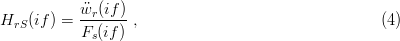
The time data records of the response were saved during the measurement and evaluated in off line mode on the control computer. The Frequency Response Function (FRF) was evaluated for each point of measurement

HrS (if ) = ¨wr(if)-, (4) Fs(if)

where i is the imaginary unit, w_r(if) is the measured acceleration in the point r in frequency domain, which was induced by excitation force F_s(if) acting in the point S. The values of the Frequency Response Functions H_rS(if) were determined as an average of the 8 measurements with 75% overlap of the windows. The length of each signal window in time domain was 64 s, the frequency range of the window was set to 10 Hz. According to the fact that the excitation force could be affected by additional dynamic forces caused e.g. by wind during the experiment and these forces could not be measured, the Operating Deflection Shapes Frequency Response Functions (ODS FRF) were evaluated. The function ODS FRF is a complex function, which can be expressed by the real and the imaginary part or by magnitude and phase functions. The magnitude function is expressed just as a frequency spectrum of the measured response but the phase function is a phase of the measured response related to the phase measured in the reference point S. The evaluation of the natural frequencies and modes of vibration of the bridges were done in the software MEScopeVES of the company Vibrant Technology, Inc.

4 Results

Because the finite element mesh was obtained from a mesh of virtual straight bridge by bending, the numerical analysis was performed on both meshes. The reason is to show the influence of apposite mesh on dynamic behaviour.

The relative difference between the calculated and measured eigenfrequencies is given in the code ČSN 73 6209 in the form

Δ = f(j)cal −-f(j)obs100 (% ) , (5) (j) f(j)cal

where f_(j)cal denotes the j-th calculated eigenfrequency and f_(j)obs denotes the j-th observed (measured) eigenfrequency. The permissible range for the relative difference has the form

r = ± (14 + -f(j)cal-) ≤ ±25 (%) . (6) f(min)cal

Table 2 summaries eigenfrequencies obtained from the numerical analysis and measured on existing structure. The relative differences and permissible ranges are also included. Question marks indicate values which were not obtained with required reliability.

Table 2: Measured and computed eigenfrequencies and circular eigenfrequencies.


j	ω_0,i (s⁻¹)		f_(j)cal (Hz)		f_(j)obs (Hz)	Δ_(j) (%)	r(%)

	straight	curved	straight	curved	measured

1	5.862073	5.211826	0.932978	0.829487	0.78	5.96	±14.7

2	6.548391	6.452192	1.042208	1.026898	0.88	14.3	±14.9

3	6.975418	6.941419	1.110172	1.104761	1.05	4.95	±15.0

4	7.251255	7.144612	1.154073	1.137100	1.23	-8.17	-15;+10

5	8.066984	7.852371	1.283900	1.249743	1.30	-4.02	±15.1

6	8.614414	9.555517	1.371026	1.520807	????	????	????

7	9.976354	9.828060	1.587786	1.564184	1.50	4.10	±15.4

8	10.960545	10.948090	1.744424	1.742442	????	????	????

9	12.502974	12.334055	1.989910	1.963025	1.80	8.30	±15.7

10	14.295015	14.079335	2.275122	2.240795	????	????	????

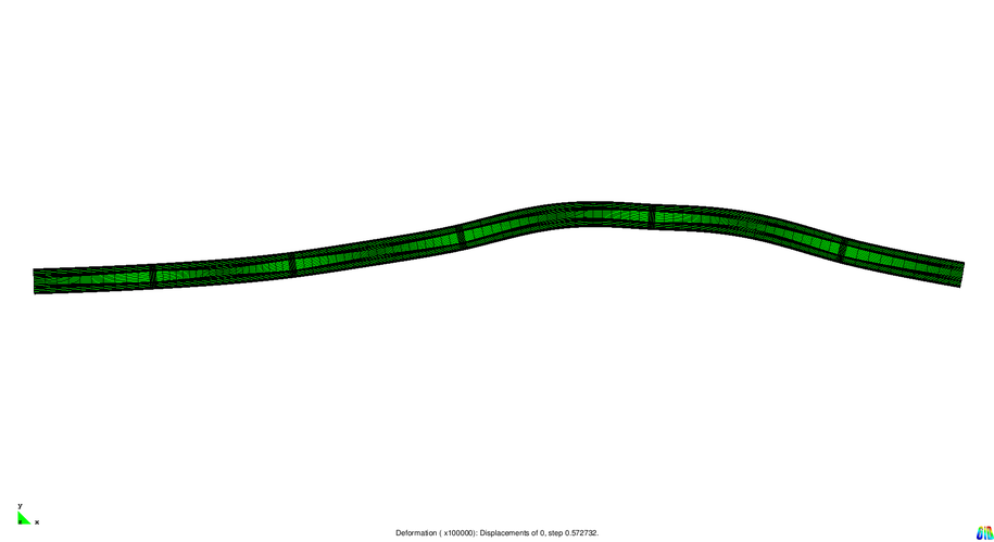
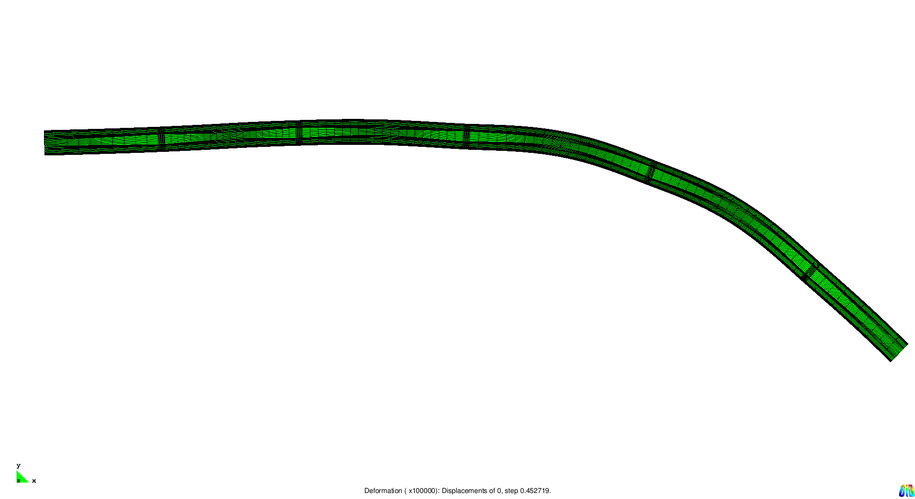
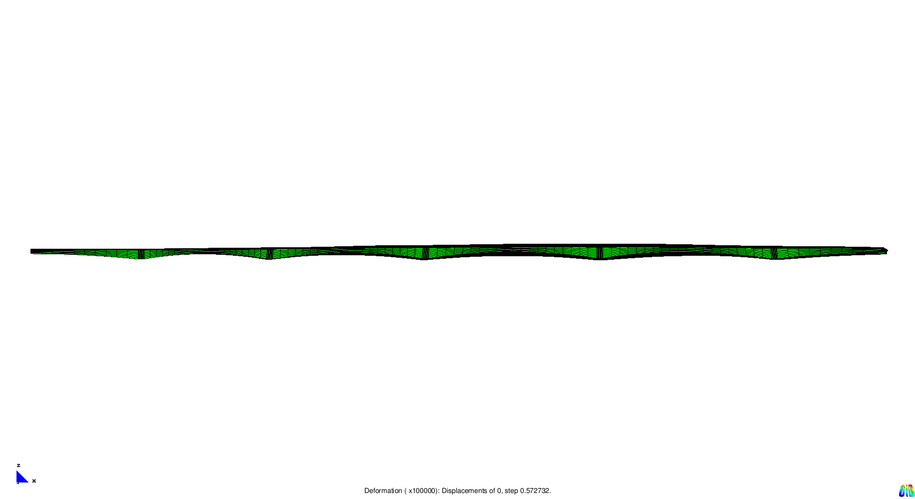
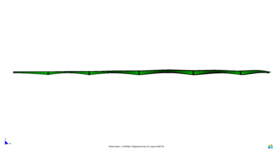
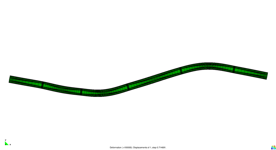
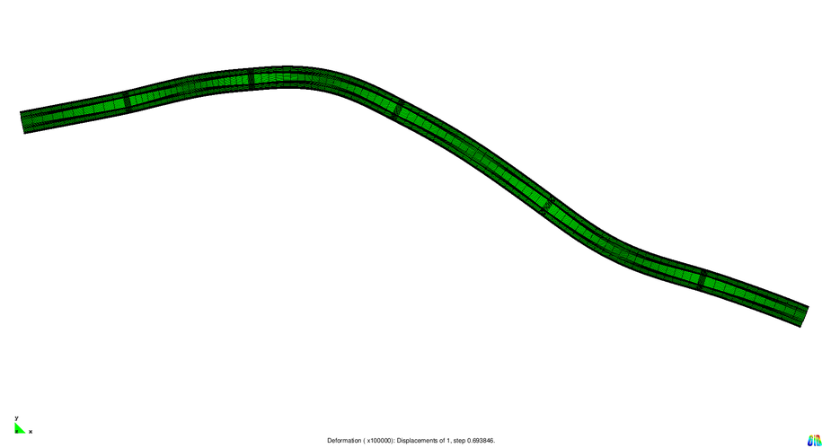
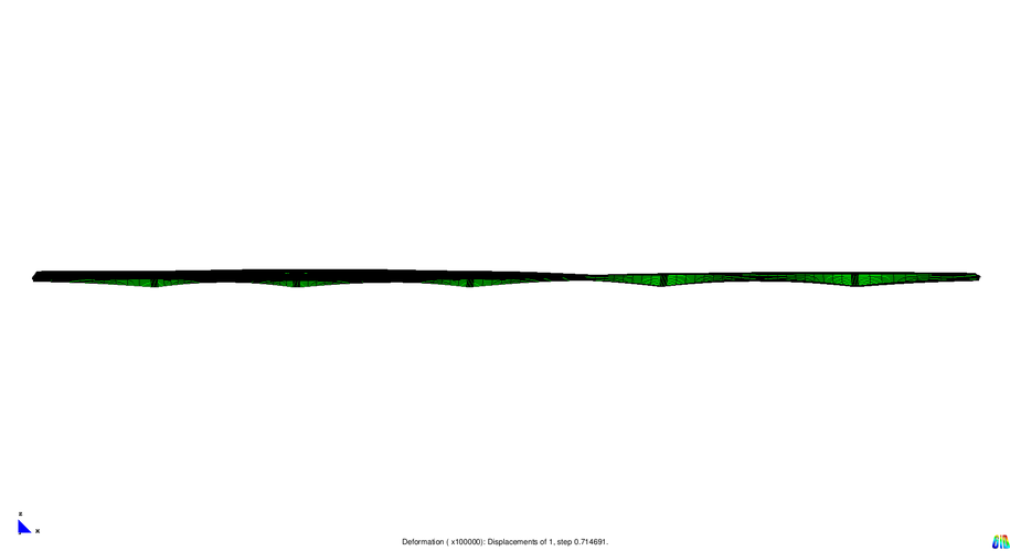
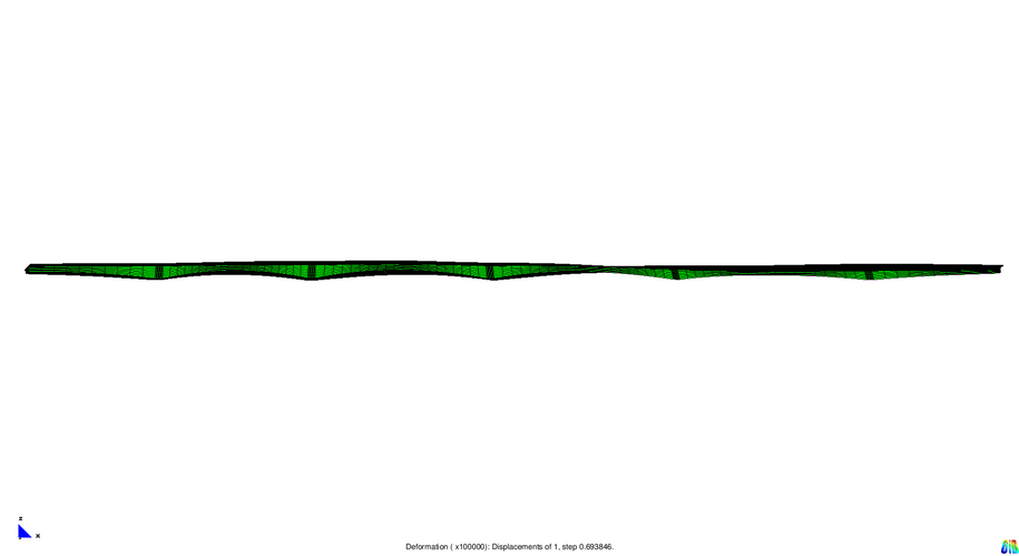
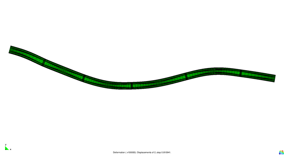
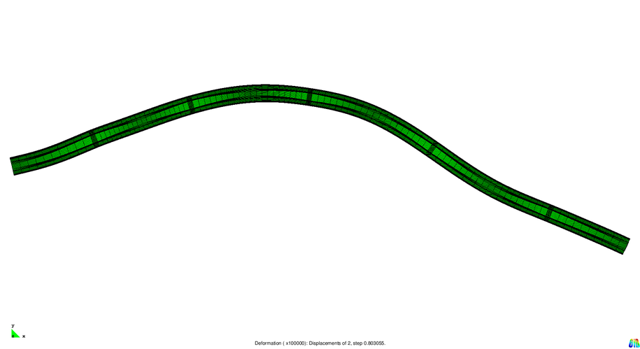
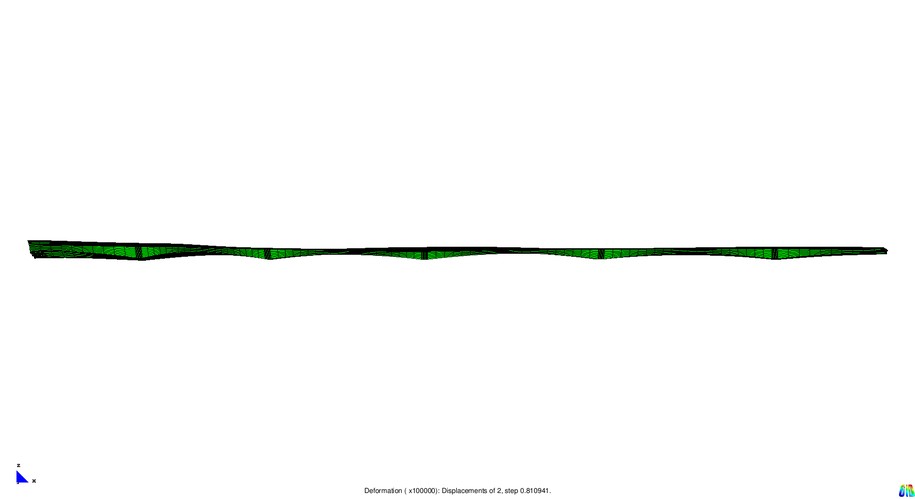
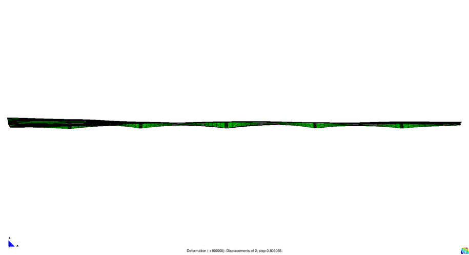
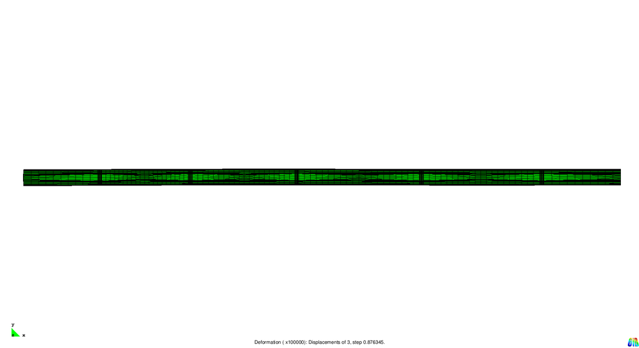
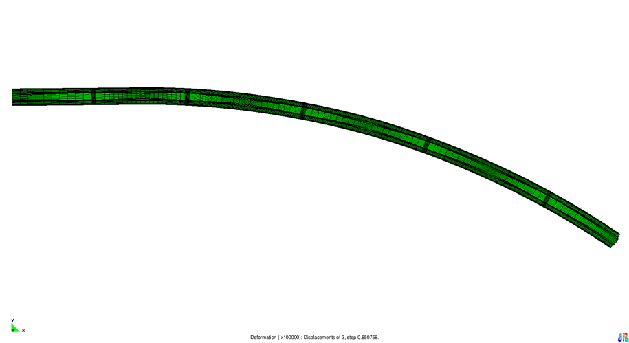
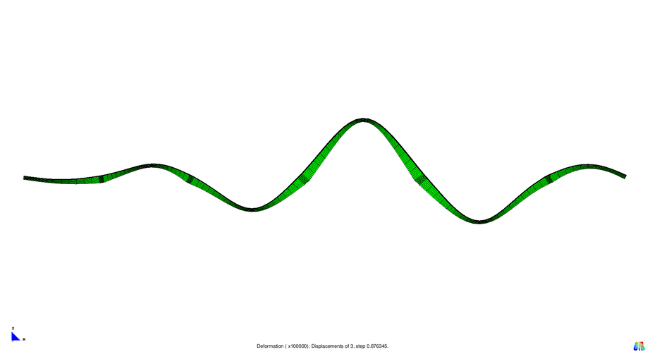
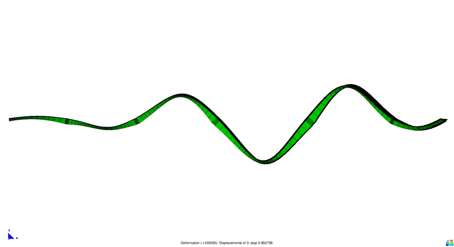
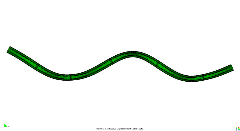
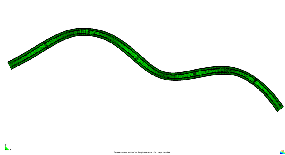
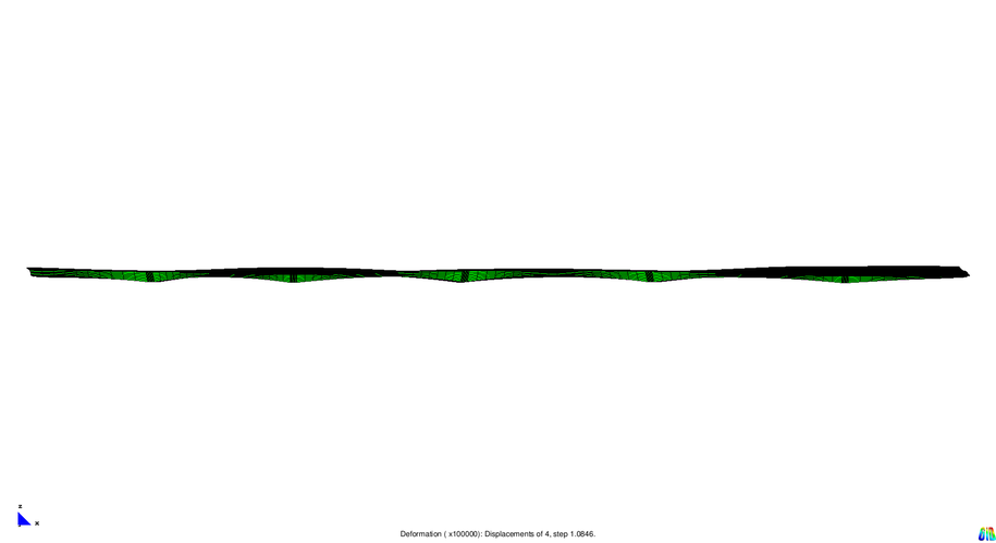
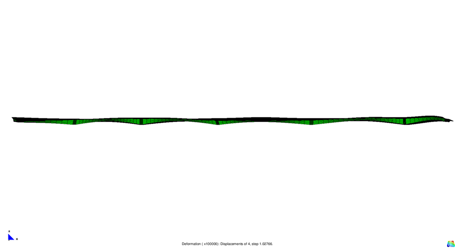
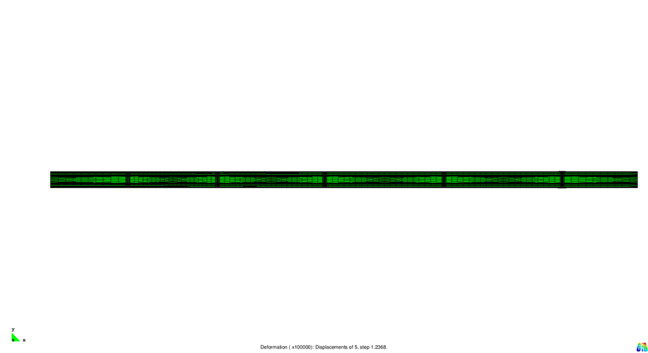
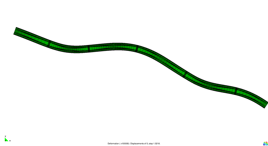
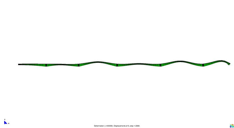
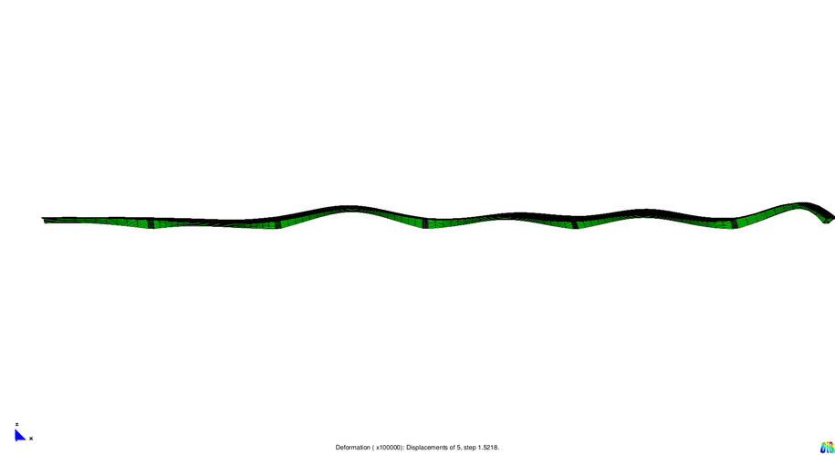
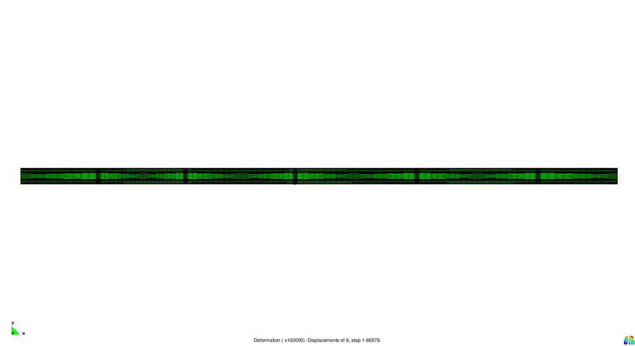
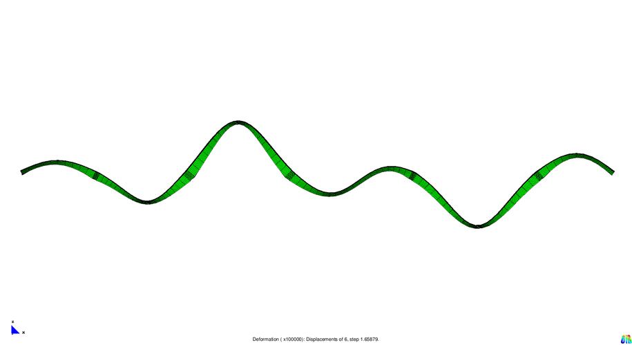
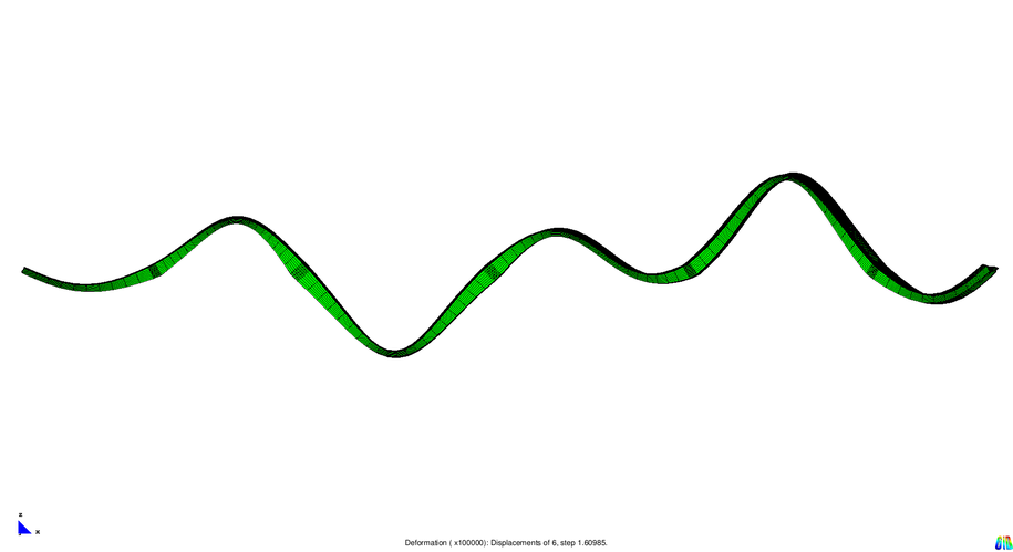
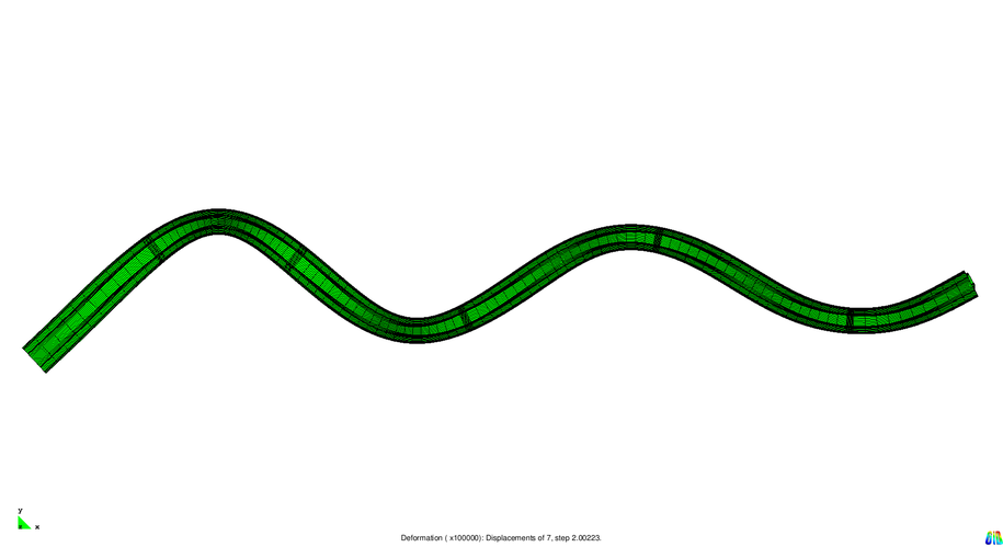
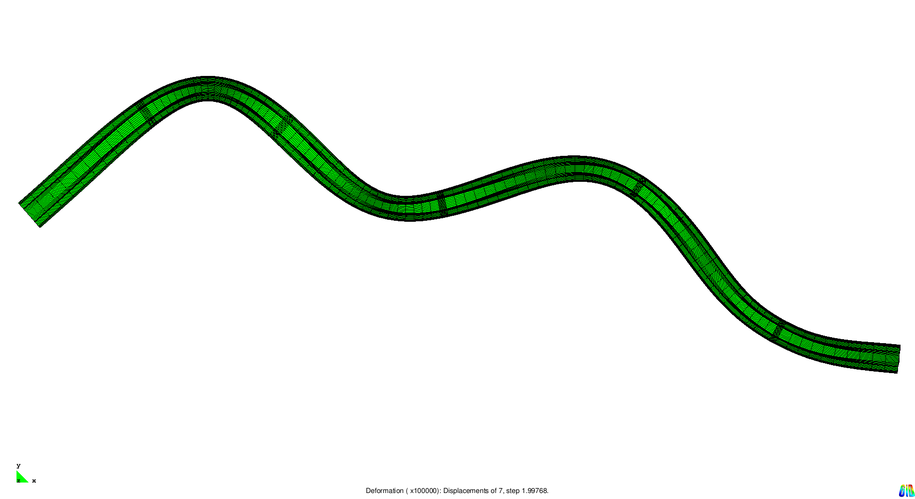
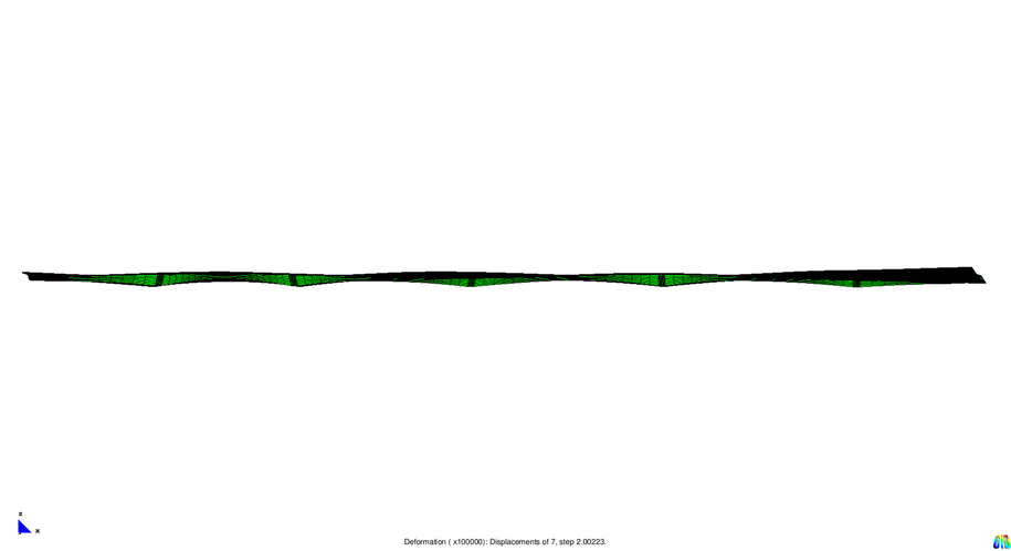
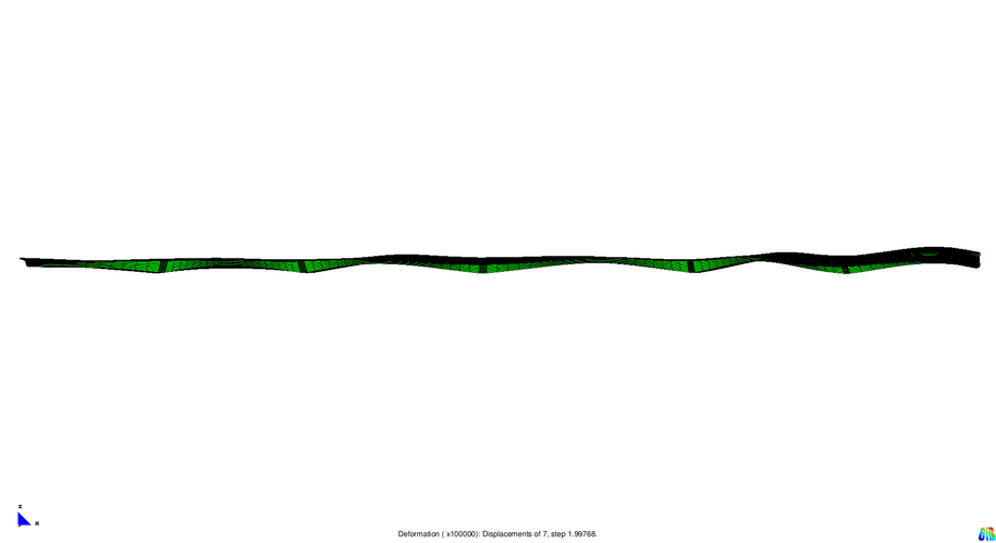
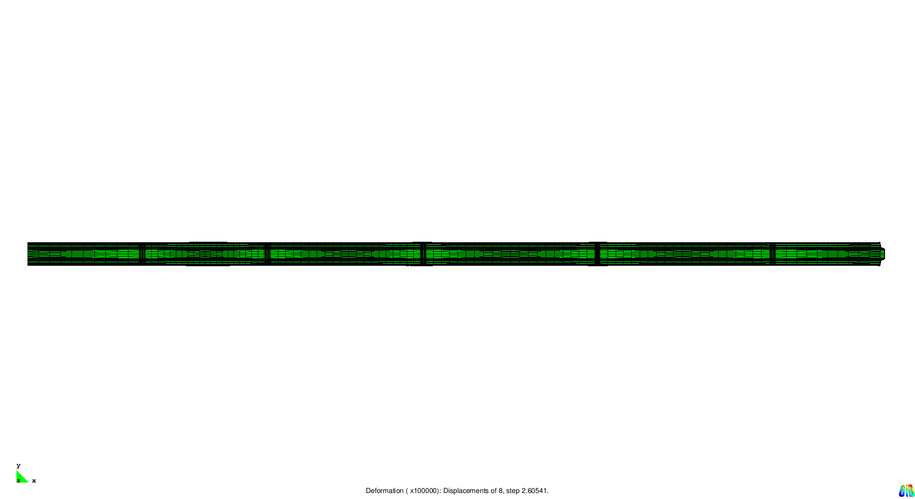
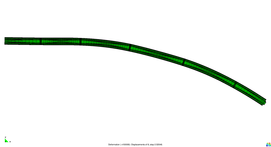
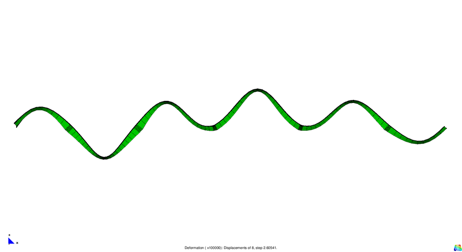
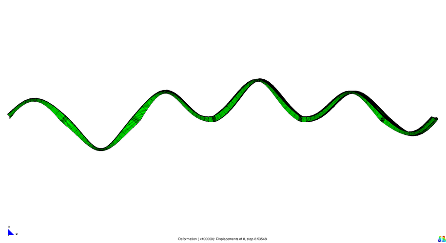
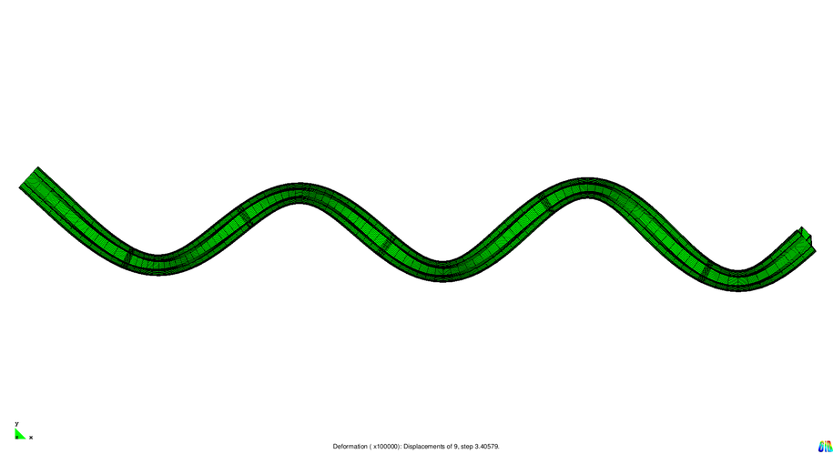
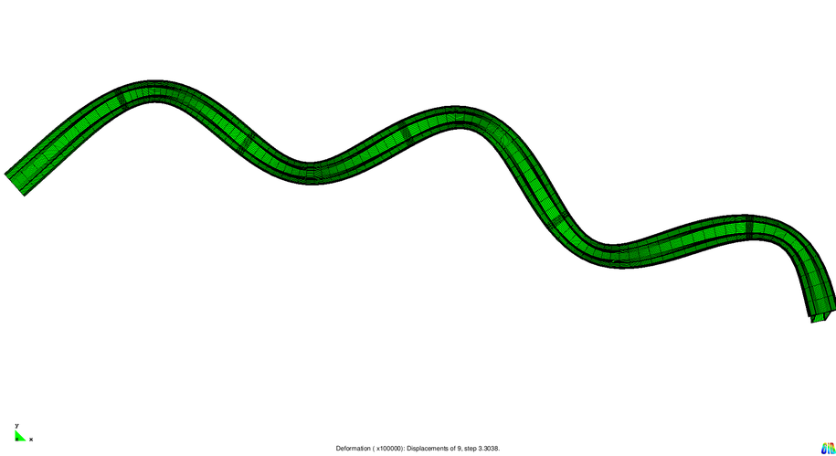
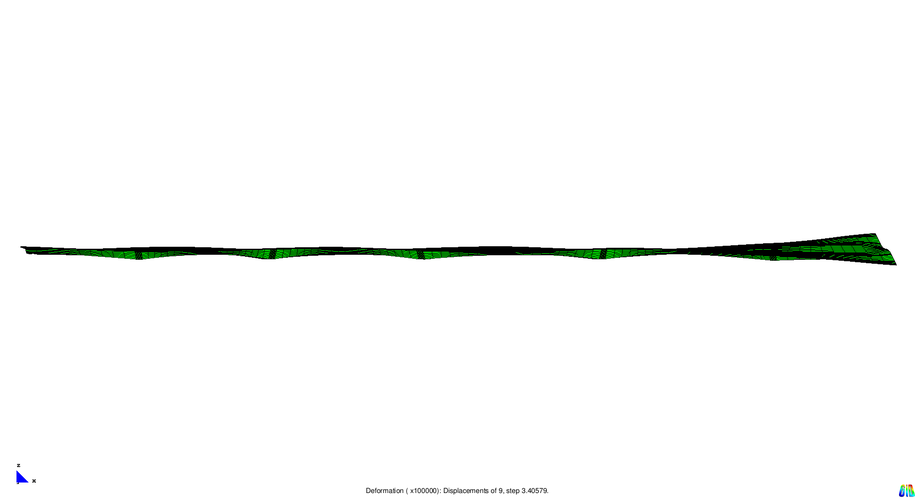
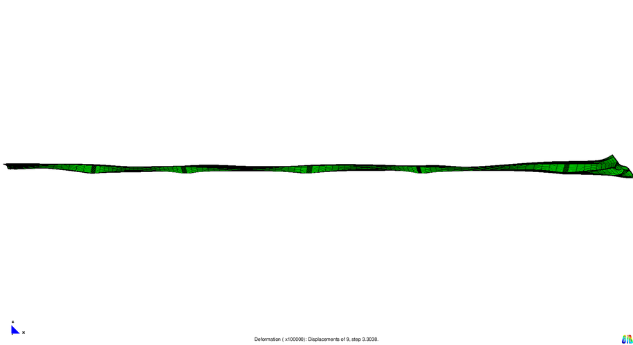
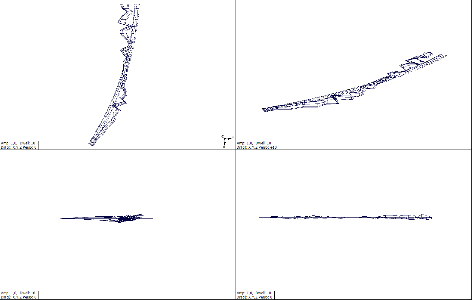
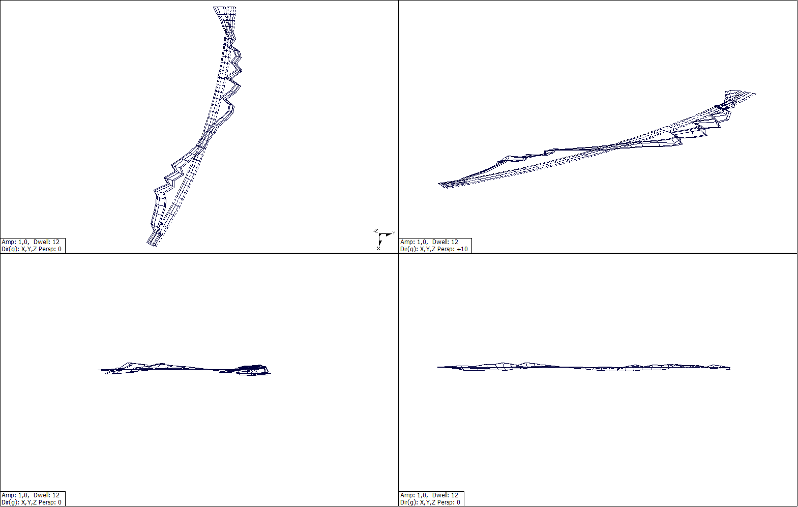
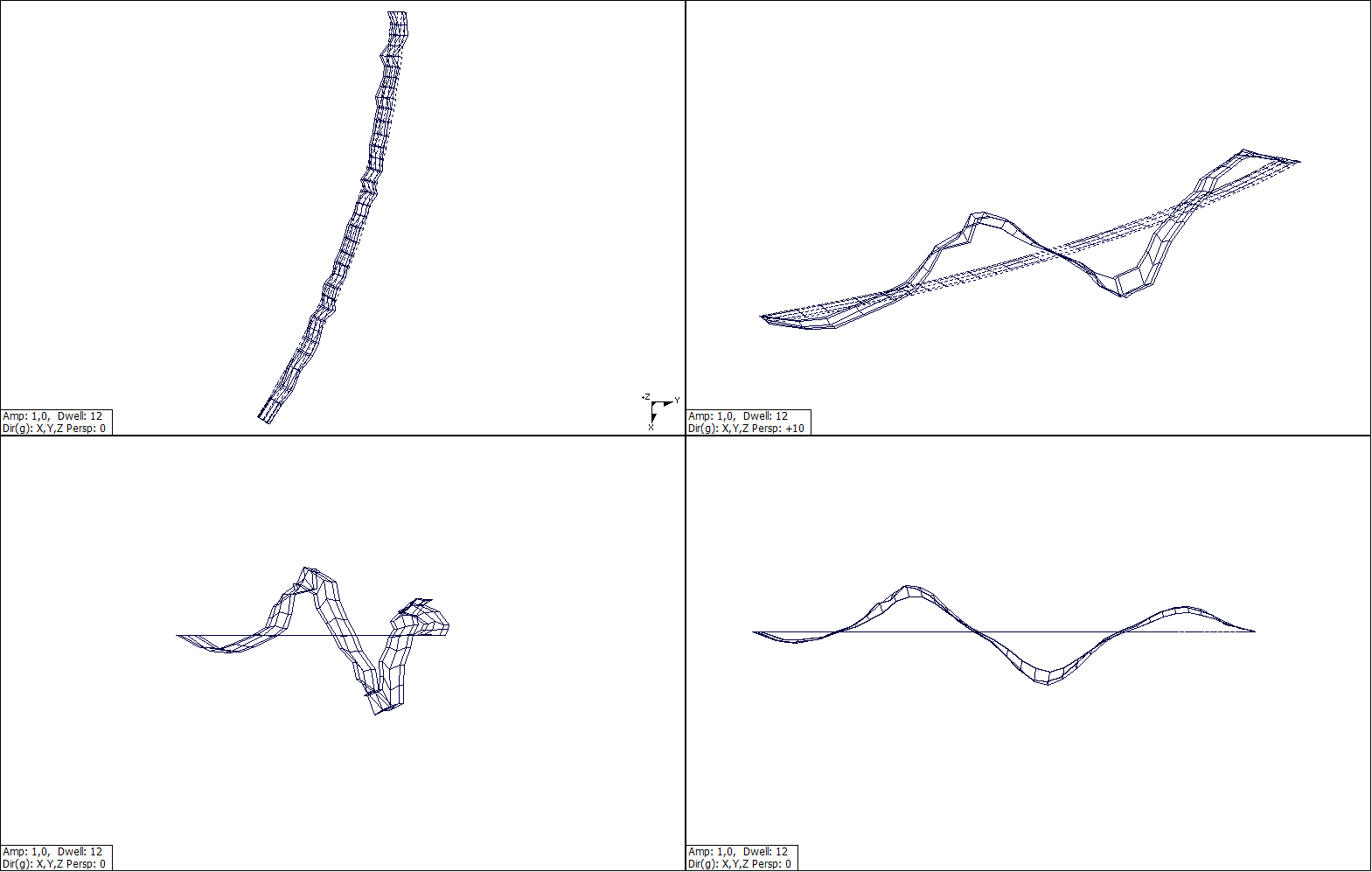
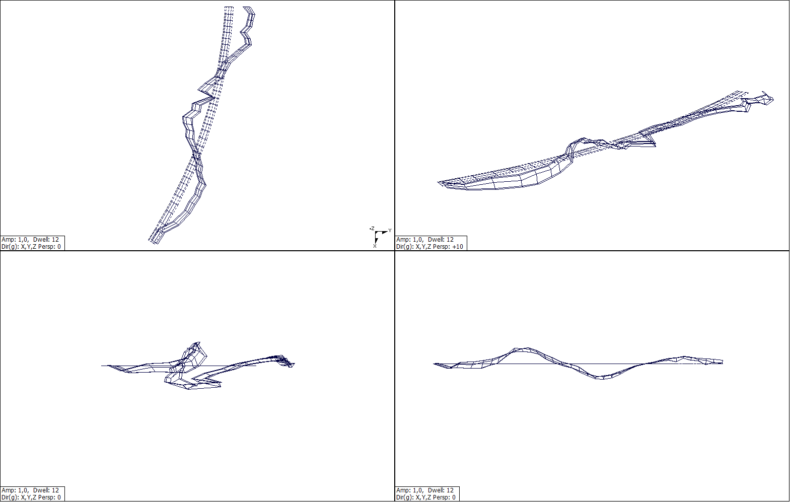
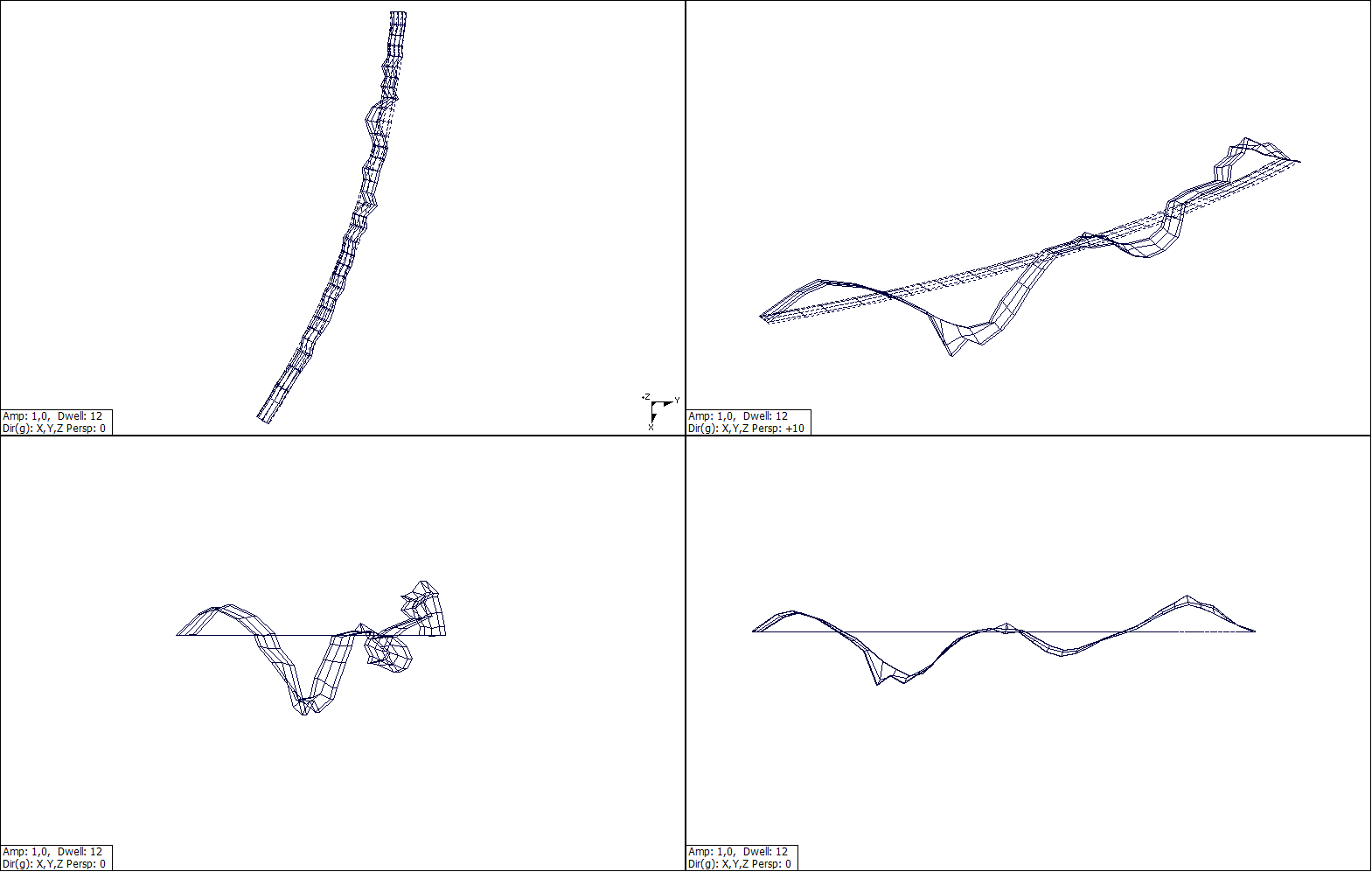
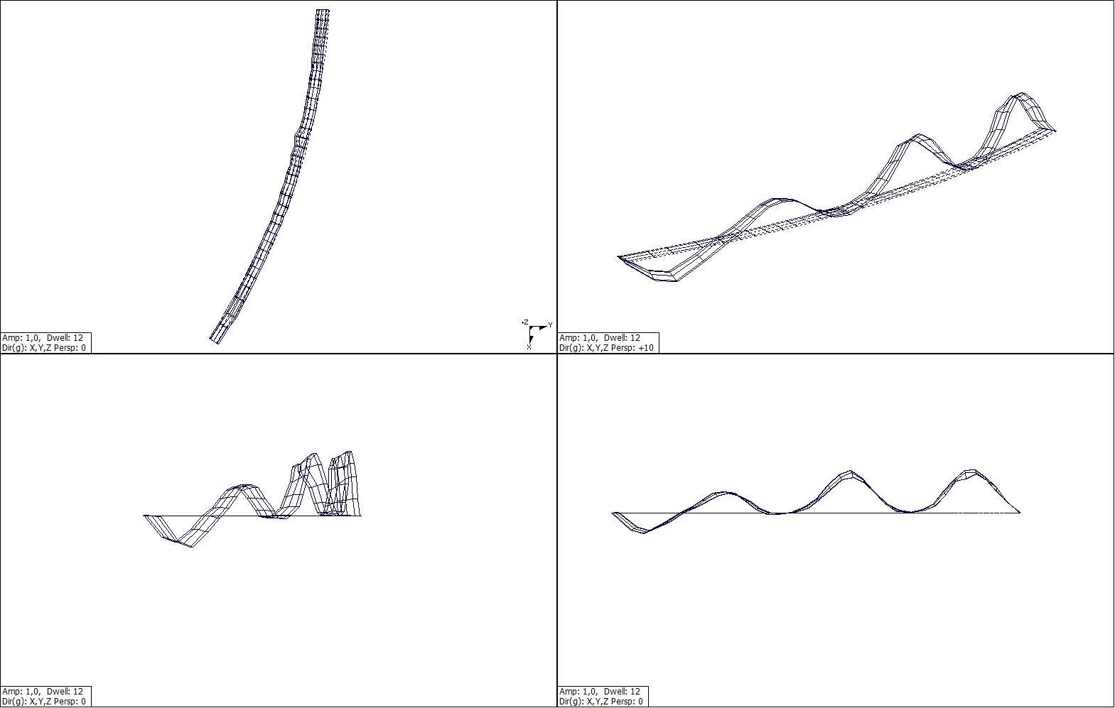
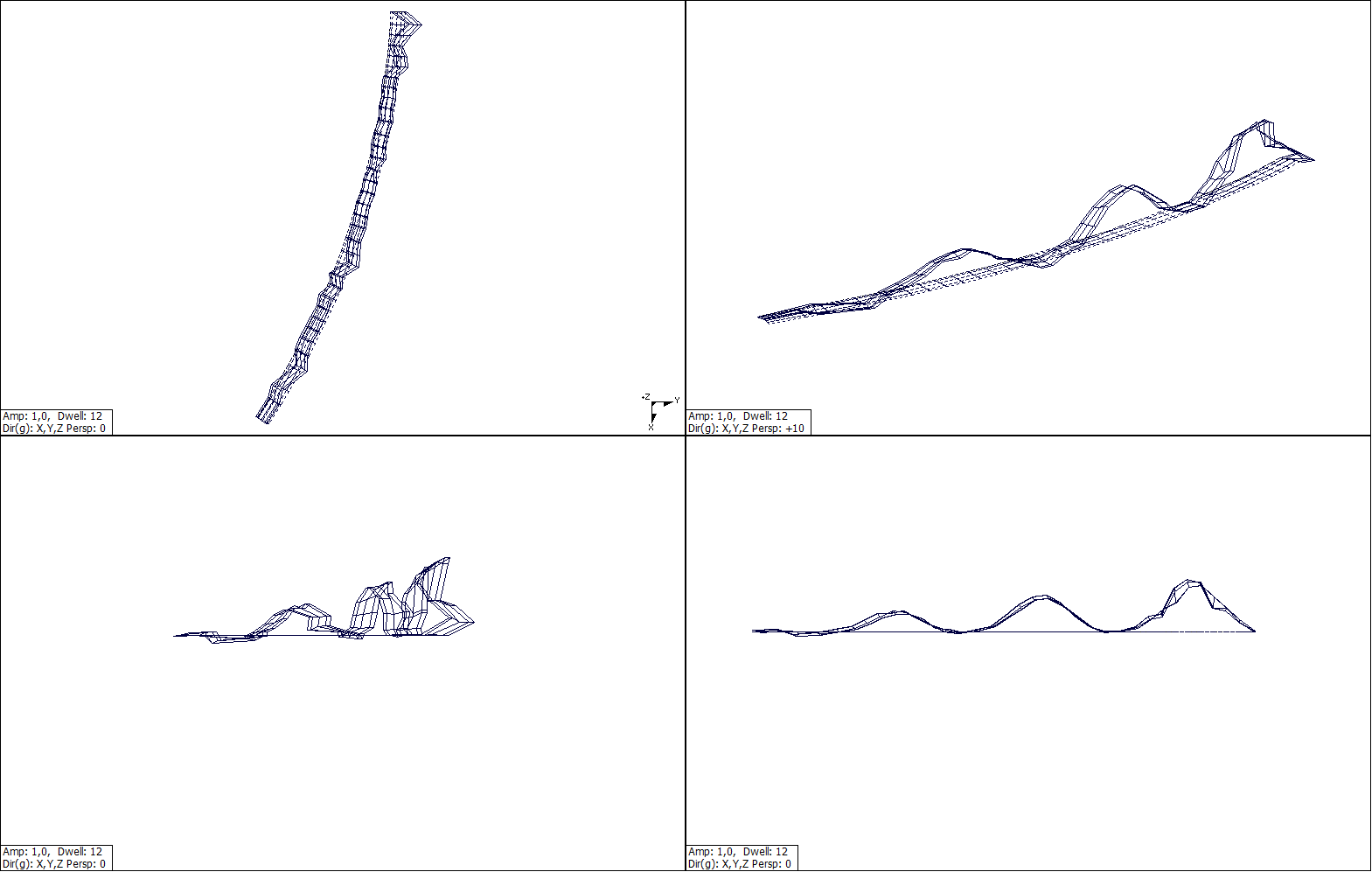
First ten calculated eigenmodes are depicted in figures 1–10. The eigenmodes of virtual straight bridge are in the left hand side of figures while the eigenmodes of the real curved bridge are in the right hand side.

Figure 1: 1st eigenmode.

Figure 2: 2nd eigenmode.

Figure 3: 3rd eigenmode.

Figure 4: 4th eigenmode.

Figure 5: 5th eigenmode.

Figure 6: 6th eigenmode.

Figure 7: 7th eigenmode.

Figure 8: 8th eigenmode.

Figure 9: 9th eigenmode.

Figure 10: 10th eigenmode.

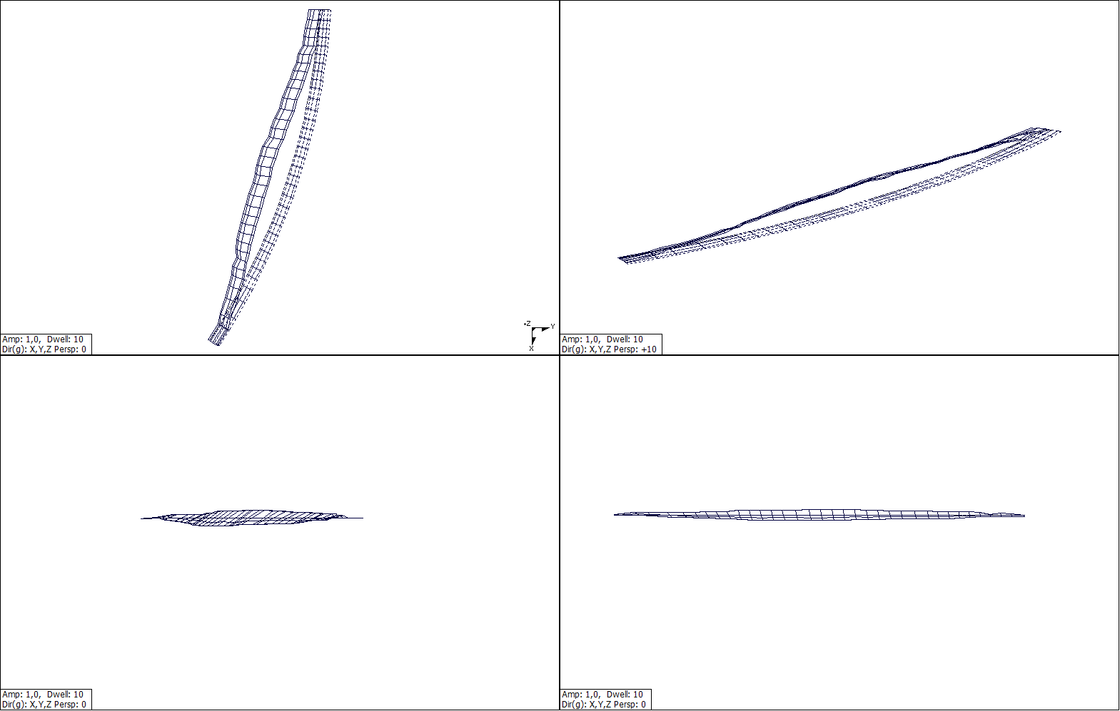
The eight natural frequencies and natural mode shapes were evaluated during an experimental modal analysis on both bridges in the frequency range from 0.5 to 2.5 Hz and the natural torsional mode with the corresponding natural frequency 4.80 Hz for the left bridge and 4.74 Hz for the right bridge. The evaluated natural modes are shown in figures 11–18.

Figure 11: 1st eigenmode.

Figure 12: 2nd eigenmode.

Figure 13: 3rd eigenmode.

Figure 14: 4th eigenmode.

Figure 15: 5th eigenmode.

Figure 16: 7th eigenmode.

Figure 17: 9th eigenmode.

Figure 18: 10th eigenmode.

5 Conclusions

The measured eigenfrequencies and eigenmodes were compared with the eigenfrequencies and eigenmodes obtained from numerical analysis based on the finite element three-dimensional model because of the curved shape of the bridges. All compared eigenfrequencies satisfy conditions given in the code ČSN 73 6209. The experimentally obtained eigenmodes contain the same number of vibration nodes and lines as the numerically obtained eigenmodes. Moreover, the vibration lines are located in the same bays of the bridges.