0.1 Plastic material models
  0.1.1 Rate Independent Plasticity
   0.1.1.1 Continuous formulation
   0.1.1.2 Discrete formulation, cutting plane method
  0.1.2 Non-smooth potentials and the subdifferential
  0.1.3 J₂ plasticity

List of Tables

0.1 Plastic material models

0.1.1 Rate Independent Plasticity

Short overview of rate independent plasticity is the aim of this section. The first part is devoted to the continuous formulation and the second one to the discrete version.

0.1.1.1 Continuous formulation

When displacements and strains are small, the additive decomposition of strain tensor is used in form

e p e p ε = ε + ε , εij = εij + εij ,

(1)

where ε (ε_ij) denote strain tensor, ε^e (ε_ij^e) stand for elastic (reversible) part of strain tensor and ε^p (ε_ij^p) mean plastic (irreversible) part of strain tensor. Stresses are calculated from the constitutive law

σ = D εe = D (ε - εp) , σij = Dijklεekl = Dijkl(εkl - εpkl) .

(2)

Strain and stress tensors are tensors of second order and their are symmetric. The set of symmetric tensors of second order will be denoted S. R^m means the m-dimensional vector space. Yield function f play important role in the theory of plasticity. It depends on stress tensor and on m parameters which are called hardening/softening parameters. Yield function is mapping from the space of symmetric tensors of second order and m-dimensional vector space into set of real numbers

f(σ, q) : S × Rm → R .

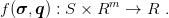(3)

There are three important cases which may occur. If the value of yield function is less than zero, material point is in elastic state. If the value of yield function is equal to zero, the material point is on the yield surface and several states may occur. Stresses and hardening parameters which results in positive value of yield function are not admissible. Stress space is defined as

E σ = {(σ, q ) ∈ S × Rm | f(σ, q ) ≤ 0} ,

(4)

elastic domain is defined as

intE = {(σ, q ) ∈ S × Rm | f(σ, q) < 0} σ

(5)

and the yield surface is defined as

∂E = {(σ, q) ∈ S × Rm | f (σ, q) = 0} . σ

(6)

Evolution of plastic strains is directed by the flow rule

p m p ˙ε = γ˙r (σ, q) , r : S × R → S , ˙εij = γ˙rij(σkl, qp) ,

(7)

where γ is the consistency parameter which always satisfy condition

˙γ ≥ 0 .

(8)

Evolution of hardening parameters is directed by the hardening rule

˙q = γ˙h (σ, q ) , h : S × Rm → Rm , ˙q = ˙γh (σ , q ) . i i kl p

(9)

Kuhn-Tucker conditions

˙γ ≥ 0 , f(σ, q) ≤ 0 , γ˙f (σ, q ) = 0

(10)

Consistency condition

˙γf˙(σ, q) = 0

(11)

Derivate of yield function with respect to time with help of constitutive relation has form

( )T ( )T ( )T ( )T f˙(σ, q ) = -∂f ˙σ + ∂f- ˙q = ∂f- D (ε˙- ε˙p ) + ∂f- ˙q . ∂ σ ∂q ∂σ ∂q

(12)

Applying flow and hardening rules one can observe

( ) ( ∂f )T ( ∂f )T ( ∂f)T ˙f(σ, q ) = --- D ˙ε - ( --- Dr + --- h) ˙γ . ∂ σ ∂ σ ∂q

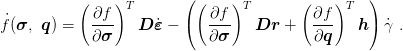(13)

Consistency parameter is expressed from condition ḟ(σ, q) = 0 in the form

( )T -∂f ∂ σ D ˙ε ˙γ = (---)T--------(----)T--- ∂f- Dr + ∂f- h ∂ σ ∂q

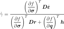(14)

Constitutive relation can be rewritten

( ) || ( )T || ˙σ = D (ε˙- ε˙p) = || D - (----)-----1---(---)----Dr ∂f- D || ε˙, |( ∂f- T ∂f- T ∂σ |) ∂σ Dr + ∂q h

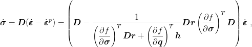(15)

where the elastoplastic stiffness matrix is defined as

( ) | ( )T | ep || ------------1----------- ∂f- || D = || D - ( ∂f )T (∂f )T Dr ∂σ D || ( --- Dr + --- h ) ∂σ ∂q

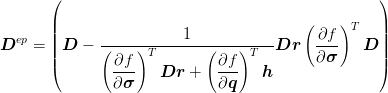(16)

and the constitutive relation for elastoplasticity can be written

ep ˙σ = D ε˙.

(17)

0.1.1.2 Discrete formulation, cutting plane method

Discrete formulation will be described on one integration point. It is assumed that n-th iteration is in equilibrium and particular variables are known. There is an increment of displacements (calculated from any iterative method for solution of nonlinear problems, e.g. Newton-Raphson or arc-length) and increments of components of strain tensor are calculated

εn+1 = εn + Δ εn .

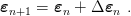(18)

The plastic strain tensor is not known at this moment and therefore the trial tensor is assumed

εpn,t+ri1al= εpn

(19)

and similarly for hardening parameters

trial q n+1 = qn .

(20)

Trial stress is computed from constitutive relation

σtrni+al1 = D (εn+1 - εp,ntr+i1al) .

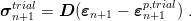(21)

Stress tensor and hardening parameters must satisfy condition

f (σtrial, qtrial) = ftrial< 0 . n+1 n+1 n+1

(22)

If the condition (22) is satisfied, the material point is in elastic domain and no plastic strain and no change of hardening parameters occur. Otherwise new consistency parameter is defined by relation

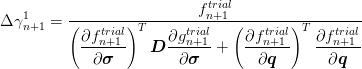1 -----------------f-trni+a1l------------------ Δ γn+1 = ( trial)T trial ( trial)T trial ∂fn+1-- D ∂g-n+1 + ∂fn+1-- ∂fn+1-- ∂σ ∂σ ∂q ∂q

(23)

New plastic strain is defined by the flow rule

trial εpn,1+1 = εpn+1 + Δ γ1 ∂gn+1- n+1 ∂σ

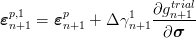(24)

and new hardening parameters are defined by hardening rule

trial q1n+1 = qn+1 + Δ γ1n+1 ∂fn+1-- ∂q

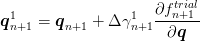(25)

New trial stress is computed from constitutive relation

1 p,1 σ n+1 = D (εn+1 - εn+1) .

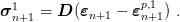(26)

Stress tensor and hardening parameters must satisfy condition

1 1 1 f(σ n+1, qn+1) = fn+1 < 0 .

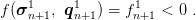(27)

If the condition (27) is not satisfied, equation (23) is used for new consistency parameter Δγ_n+1².

Algorithm can be summarized in the following table


1.	increment of displacements	Δu_n is obtained

	total strain	ε_n+1 = ε_n + Δε_n

2.	initialization of variables	k = 0

	plastic strain	ε_n+1^p,k = ε_n^p

	hardening parameters	q_n+1^k = q_n

	consistency parameter	γ_n+1^k = γ_n


3.	new stress	σ_n+1^k = D(ε_n+1 -ε_n+1^p, k)

4.	yield function	f_n+1^k = f(σ_n+1^k, q_n+1^k)

5.	admissibility check	if f_n+1^k < 0 go to step 1.

6.	consistency parameter	Δγ_n+1^k =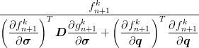

7.	new plastic strain	ε_n+1^p, k+1 = ε_n+1^p, k + Δγ_n+1^k

8.	new hardening parameters	q_n+1^k+1 = q_n+1^k + Δγ_n+1^k

9.	new consistency parameter	γ_n+1^k+1 = γ_n+1^k + Δγ_n+1^k

10.		go to step 3.

0.1.2 Non-smooth potentials and the subdifferential

[?] if the potential Ψ is not differentiable, it is called non-differentiable, the function Ψ is called a pseudo-potential or generalized potential

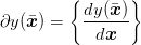
Let us consider a scalar function y : Rⁿ → R. The subdifferential of y at a point x is the set

n T n ∂y(¯x ) = {s ∈ R |y(x ) - y (¯x) ≥ s (x - ¯x),∀x ∈ R }

(28)

If the set ∂y is not empty at x, the function y is said to be subdifferentiable at x. The elements of ∂y are called subgradients of y. If the function y is differentiable, then the subdifferential contains a unique subgradient which coincides with the derivative of y

{ } dy(¯x-) ∂y (¯x) = dx

(29)

Plastic flow with subdifferentiable flow potentials

Let Ψ be a pseudo-potential which is subdifferentiable function of σ and A. The plastic flow rule has the form

˙εp = ˙γN

(30)

where

N = ∂-Ψ- ∂ σ

(31)

for differentiable function Ψ and

N ∈ ∂σΨ

(32)

for subdifferentiable function Ψ. N is a subgradient. Similarly, for hardening law

H = - ∂-Ψ- ∂A

(33)

for differentiable function Ψ and

H ∈ - ∂A Ψ

(34)

for subdifferentiable function Ψ.

An alternative definition of the plastic flow rule with non-smooth potentials is a linear combination of distinct normals (N₁,N₂,…,N_n). The flow rule has the form

∑n ˙εp = ˙γiN i i=1

(35)

Kinematic hardening [?], str. 185

von Mises-type yield surface

∘ ------------- Φ (σ,β ) = 3J2(η(σ, β)) - σy

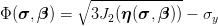(36)

where

η(σ,β ) = s(σ ) - β

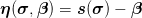(37)

is the relative stress tensor and β is the back-stress tensor.

Isotropic scalar-valued function

Let be the space of symmetric tensors in an n-dimensional space. A scalar-valued function of a symmetric tensor ϕ(X) : ⊂→ R is called isotropic if

ϕ(X ) = ϕ(QXQT )

(38)

for all rotations Q.

In three-dimensional space, a scalar function of a symmetric tensor is isotropic if and only if it admits the representation

ϕ (X ) = ¯ϕ(I1(X ),I2(X ),I3(X )) ∀X ∈ L

(39)

where I_i(X) are the principal invariants. The principal invariants themselves are isotropic functions. Another representation of ϕ(X) has the form

ϕ(X ) = ϕˆ(λ1(X ),λ2(X ),λ3(X )) ∀X ∈ L

(40)

where λ_i(X) are the eigenvalues of X. There are the following symmetries

ˆϕ(λ1,λ2,λ3) = ϕˆ(λ2,λ1,λ3) = ˆϕ(λ1,λ3, λ2)

(41)

Unlike the isotropically hardening von Mises model, the function

∘ ------------- Φ (σ,β ) = 3J2(η(σ, β)) - σy

(42)

is not an isotropic function of the stress tensor for kinematically hardened states β≠0.

0.1.3 J₂ plasticity

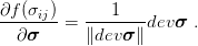
Yield function is defined in tensorial form as

∘ --------------- ∘ -- f (σij) = σijσij - 1-(σii)2 - 2σY , 3 3

(43)

where σ_ij denotes the stress tensor and σ_Y yield stress. Derivative of yield function with respect to stress tensor can be writen in tensorial form as

( ) ∂f-(σij)- -------1--------- 1- ∂σij = ∘ --------1------ σij - 3σllδij σijσij - -(σii)2 3

(44)

or in the matrix form as

∂f (σij) 1 --------= -------dev σ . ∂σ ∥devσ ∥

(45)

Contents