1 Heat transport
1.1 Non-stationary heat transport
2 Coupled transport of several physical quantities
2.1 General scheme of coupled transport of several physical quantities
2.2 Coupled heat and moisture transport
  2.2.1 Künzel model
   2.2.1.1 Theoretical description
   2.2.1.2 Matrix notation
   2.2.1.3 Discretization
2.3 Coupled heat, moisture and salt transport
  2.3.1 Černý model
   2.3.1.1 Theoretical description
   2.3.1.2 Matrix notation
   2.3.1.3 Discretization
3 Time integration methods
3.1 Generalized Trapezoidal Method

List of Tables

3.1 v-version of the generalized trapezoidal method.
3.2 d-version of the generalized trapezoidal method.

Chapter 1
Heat transport

1.1 Non-stationary heat transport

Non-stationary heat transport is described in three-dimensional space. One or two-dimensional problems could be obtained easily by reduction of the sums used in the exposition.

Let a three-dimensional domain Ω be assumed. Coordinates of points in the domain Ω are denoted x_i in component notation or x in vector notation. Time is denoted t. The amount of heat which flows through in the normal direction to an unit area (one meter squared) per unit time (one second) is called the heat flux density and is denoted q_n(x_i,t), where the subscript n indicates the normal direction. The heat flux denisity is expressed in J/(m²s). In a general coordinate system, the density of heat flux is a vector and it is denoted q(x,t). The amount of heat stored in a unit volume is s(x,t) (J/m³).

The heat balance equation has the form

3 ∑ ∂qi-+ ∂s-= z , (1.1) i=1 ∂xi ∂t

where z denotes the source of heat per unit volume and unit time (J/(m³s)). The stored heat can be expressed in the form

s = ϱcT , (1.2)

where ρ stands for the density of material (kg/m³), c expresses the heat capacity (J/(kg K)) and T is the temperature (K). The heat flux density is proportional to the gradient of temperature which is denoted g. The relationship between the vectors q and g is called the Fourier law and it has the form

3 3 q = - ∑ d g = - ∑ d ∂T--, (1.3) i j=1 ij j j=1 ij∂xj

where d_ij stands for the heat conductivity coefficients. d_ij are components of the heat conductivity tensor. Usually, the off-diagonal components of d_ij are equal to zero. Moreover, an isotropic material is described by a single heat conductivity d and the conductivity tensor has the form

dij = dδij , (1.4)

where δ_ij is the Kronecker delta.

The flux in the direction of a normal vector n_i could be expressed with the help of the heat flux density q_i in the form

∑3 ∑3 ∑3 ∂T qn = qini = - nidij----. (1.5) i=1 i=1 j=1 ∂xj

Let boundary of the domain Ω be denoted Γ. The boundary is a union of four parts Γ_p, Γ_f, Γ_t and Γ_r. Dirichlet boundary condition (prescribed value) is prescribed on Γ_p, Neumann boundary condition (prescribed flux density) is prescribed on Γ_f, Newton (Cauchy, Robin) boundary condition (transmission) is prescribed on Γ_t and radiation boundary condition is prescribed on Γ_r.

For all internal points of the domain Ω, the governing equation has the form

3 ( 3 ) ∑ -∂--(∑ d -∂T-) + z = ρc∂T- , (1.6) i=1 ∂xi j=1 ij∂xj ∂t

where z denotes the source of heat per unit volume and unit time (J/(m³s)), ρ stands for the density of material (kg/m³) and c expresses the capacity (J/(kg K)). Boundary conditions are in the form

∀x ∈ Γ p : T(x, t) = p (x, t) , (1.7) ∀x ∈ Γ f : qn(x,t) = w (x, t) , (1.8) ∀x ∈ Γ t : qn(x,t) = κ(T (x,t) - Text(x, t)) , (1.9) ∀x ∈ Γ r : qn(x,t) = σε(T 4(x,t) - T4ext(x, t)) (1.10 )

and the initial condition is in the form

T (x,0 ) = e(x ) .

(1.11)

The problem has non-homogeneous boundary conditions and will be transformed into problem with homogeneous conditions. The function T is split into two functions

T (x,t) = ˜T (x,t) + Tˆ(x,t)

(1.12)

which satisfy the following conditions

∀x ∈ Γ p : ˜T (x,t) = 0 , (1.13 ) ˆT (x,t) = p(x, t) , (1.14 ) ˆT(x, 0) = e(x ) . (1.15 )

It has to be emphasized that the initial and boundary conditions have to be consistent

∀x ∈ Γ : p(x,0) = e(x ) . (1.16 ) p

The governing equation (1.6) is multiplied by a test function phi which satisfies the homogeneous Dirichlet boundary conditions and the equation is integrated over the domain Ω (this is Galerkin method). Taking into account also relationship (1.12), the following equation is obtained

( ) ∫ ∑3 ∑3 ( ˜ ˆ ) ∫ ∫ ( ˜ ˆ) ϕ -∂--( dij ∂T--+ -∂T- ) dΩ + ϕz dΩ = ϕ ρc ∂T-+ ∂T- dΩ (1.17 ) Ω i=1∂xi j=1 ∂xj ∂xj Ω Ω ∂t ∂t

The first term of (1.17) can be modified

( ) ∫ ∑3 ∂ ∑3 ∂ (˜T + ˆT ) ϕ ----( dij----------) d Ω = (1.18 ) Ω i=1 ∂xi( j=1 ∂xj ) ∫ ∑3 ∑3 ˜ ˆ ∫ ∑3 ∑3 ˜ ˆ ϕni ( dij∂(T-+--T)) dΓ - ∂ϕ-dij∂(T-+--T)d Ω (1.19 ) Γ i=1 j=1 ∂xj Ωi=1j=1 ∂xi ∂xj

The boundary integral can be reformulated with the help of (1.5) and (1.12) into the form

∫ ∑3 (∑3 ˜ ˆ ) ∫ ∫ ϕni ( dij∂-(T--+-T)-) d Γ = - ϕw dΓ f + - ϕ κ(˜T + Tˆ- Text)dΓ t + Γ i=1 j=1 ∂xj Γ f Γ t ∫ + - ϕσε((˜T + Tˆ)4 - T4ext)dΓ r (1.20 ) Γ r

Equation (1.17) could be rewritten to the form

∫ ∫ ˜ ˆ ∫ ˜ ˆ 4 4 Γ - ϕw dΓ f + Γ - ϕκ (T + T - Text)dΓ t + Γ - ϕσ ε((T + T) - Text)d Γ r - f∫ t ∫ ∫ r ( ) ∑3 ∑3 ∂-ϕ- ∂-(T˜-+-ˆT)- ∂T˜ ∂-ˆT - Ω ∂xi dij ∂xj dΩ + Ω ϕzdΩ - Ω ϕρc ∂t + ∂t dΩ = 0 . (1.21 ) i=1 j=1

The continuous functions from the previous relations are discretized by the finite element method in the following form

˜ [d] T = N d , (1.22 ) Tˆ = N [e]e , (1.23 ) [ϕ] ϕ = N ϕ , (1.24 ) w = N [w]w , (1.25 ) [z] z = N z , (1.26 ) Text = N [u]u , (1.27 ) grad T˜ = B [d]d , (1.28 ) [e] grad Tˆ = B e , (1.29 ) grad ϕ = B [ϕ]ϕ , (1.30 )

where

d	is the vector of unknown nodal temperatures,
e	is the vector of initial temperature in Ω and prescribed temperature on Γ_p,
ϕ	is the vector of nodal values of the test function,
w	is the vector of nodal values of prescribed heat flux densities on part Γ_f,
z	is the vector of nodal values of heat source,
u	is the vector of nodal values of temperature of external environment prescribed on part Γ_t,
N^[d]	is the matrix of basis (approximation) functions for temperature,
N^[e]	is the matrix of basis (approximation) functions for initial and prescribed temperature,
N^[ϕ]	is the matrix of basis (approximation) functions for the test function,
N^[w]	is the matrix of basis (approximation) functions for prescribed heat density flux on Γ_f,
N^[z]	is the matrix of basis (approximation) functions for the heat source,
N^[u]	is the matrix of basis (approximation) functions for temperature of external environment prescribed on Γ_t

After substitution of the previous approximation (1.22-1.30) to equation (1.21), the following equation is obtained

∫ ( - ϕT (B [ϕ])TDB [d]d - ϕT(B [ϕ])T DB [e]e + ϕT (N [ϕ])TN [z]z - (1.31 ) Ω ∫ - ϕT (N [ϕ])TρcN [d]d˙- ϕT(N [ϕ])TρcN [e]u ˙)dΩ - ϕT (N [ϕ])T N [w ]wd Γ - Γ f f ∫ ( T [ϕ]T [d] T [ϕ]T [e] T [ϕ]T [u] ) - ϕ (N ) κN d + ϕ (N ) κN e - ϕ (N ) κN u dΓ t = 0 . Γ t

Vector ϕ can be factored out from all terms and new form is obtained

(∫ ( ϕT - (B [ϕ])T DB [d]d - (B [ϕ])TDB [e]e + (N [ϕ])TN [z]z- Ω ∫ [ϕ] T [d]˙ [ϕ] T [e]) [ϕ] T [w] - (N ) ρcN d - (N ) ρcN ˙e dΩ - Γ f(N ) N wd Γ f- (1.32 ) ∫ ( ) ) - (N [ϕ])TκN [d]d + (N [ϕ])TκN [e]e - (N [ϕ])TκN [u]u dΓ t = 0 . Γ t

The following matrices and vectors are defined

∫ K [T] = (B [ϕ])T DB [d]dΩ (1.33 ) ∫Ω K [e] = (B [ϕ])T DB [e]dΩ (1.34 ) ∫Ω [T t] [ϕ]T [d] K = Γ t(N ) κN dΓ (1.35 ) ∫ K [et] = (N [ϕ])TκN [e]dΓ (1.36 ) ∫Γ t C = (N [ϕ])TϱcN [d]dΩ (1.37 ) ∫Ω [e] [ϕ] T [e] C = Ω (N ) ϱcN dΩ (1.38 ) ∫ [ϕ] T [z] M = Ω (N ) N dΩ (1.39 ) ∫ f [f] = (N [ϕ])T N [w]dΓ w (1.40 ) ∫Γ f f[t] = (N [ϕ])TκN [u]dΓ u (1.41 ) Γ t f [z] = M z (1.42 )

The balance equation with the previous notation has the form

( ) ( ) K [T] + K [Tt] d + C d˙= f[z] - K [e] + K [et] e - C [e]˙e - f[f] + f [t] . (1.43 )

Approximation functions for continuous functions are usually identical, therefore the following relationship is valid

N [d] = N [e] = N [ϕ] = N [z] = N [h] = N [u] . (1.44 )

The notation (1.33-1.42) can be simplified to the form

[T] ∫ T K = ΩB DBd Ω (1.45 ) [Γ ] ∫ T K = N κN dΓ (1.46 ) ∫Γ t C = N TκN dΩ (1.47 ) ∫Ω M = N TN d Ω (1.48 ) ∫Ω [f] T f = Γ N N dΓ w (1.49 ) ∫ f f[t] = N TκN dΓ u (1.50 ) Γ t f[z] = M z (1.51 )

The balance equation with the previous notation (1.45-1.51) has the form

( ) ( ) K [T] + K [Γ ] d + C ˙d = f [z] - K + K [Γ ] e - C ˙u - f [f] + f [t] . (1.52 )

Chapter 2
Coupled transport of several physical quantities

In chapter 1, transport of the heat energy is described. There is a single physical quantity transported (the energy), a single balance equation (the energy balance equation (1.6)) and a single unknown function (the temperature T). In the case of two or more transported physical quantities, the appropriate number of balance equations and unknown functions is needed. Coupled heat and moisture transport is an example of transport of heat energy and mass which could be expressed in the form of moisture. Two unknown functions are used in such models, the temperature and the relative humidity (or volumetric moisture content).

2.1 General scheme of coupled transport of several physical quantities

Let a general coupled transport of m physical quantities be assumed in a domain Ω ⊂ R^d which is from the d-dimensional space. The quantities are described by functions v^[j](x_i,t) which depend on spatial coordinates x (in the vector notation) or x_i (in the index notation) and time t. The quantites can be collected in the vector

( ) v[1](x, t) || v[2](x, t) || v(x, t) = || .. || . (2.1) ( . ) v[m ](x, t)

Flux density of the j-th quantity in the direction defined by an unit vector n (unit means that size of the vector is equal to one) is denoted by q_n^[j]. The flux density of the j-th quantity in a general coordinate system is a vector denoted q^[j](x,t) or q_i^[j](x_k,t). The flux density vector q^[j](x,t) contains d components. The vectors q^[j](x,t) can be collected in a new larger vector

( q[1](x,t) ) | [2] | q(x,t) = || q (x,t) || (2.2) |( ... |) q[m ](x, t)

which contains d.m components. Flux density of the j-th quantity in the direction defined by an unit vector n can be expressed in the form

i=d [j] ∑ [j] qn (x,t) = qi (xk,t)ni . (2.3) i=1

Gradients of the physical quantities can be written in the form

[j] [j] [j] g = grad v (x,t) = ∇v (x,t) , (2.4) [j] ∂v[j](xk,t)- gi = ∂xi . (2.5)

The gradients can be also collected in a new larger vector

( g[1](x,t) ) | [2] | g(x,t) = || g (x,t) || (2.6) |( ... |) g[m ](x, t)

which contains d.m components.

The flux densities are related with the gradients of the physical quantities by the constitutive relationships. In linear case, the flux densities have the form

k=m q[j] = - ∑ D [jk]g[k] , (2.7) k=1 k=m r=d [k] q[j] = - ∑ ∑ D [jk]∂v--(xs,t)-. (2.8) i k=1 r=1 ir ∂xr

Each constitutive matrix D^[jk] contains d rows and d columns. The components of D^[jk] are called conductivity coefficients. The constitutive relationships (2.7) can be written in the compact vector–matrix form

q(x, t) = - Dg , (2.9)

where

( [11] [12] [1m ] ) | D D ... D | || D [21] D [22] D [2m ] || D = || .. .. .. || . (2.10 ) ( .[m1] [m2 ] . .[mm ] ) D D ... D

The matrix D contains md rows and md columns. Combining (2.3), (2.7) and (2.8), flux density of the j-th quantity in the direction defined by an unit vector n can be rewritten

( )T [j] k=∑m [jk] [k] i=∑d k∑=m r=∑d [jk]∂v[k](xs,t) qn (xs,t) = - D g n = - D ir ---∂x-----ni . (2.11 ) k=1 i=1 k=1 r=1 r

Balance equation for the j-th variable has the form

∂s[j] -----+ div q[j] = z[j] , (2.12 ) ∂t ∂s[j]- i∑=d∂q-[j] [j] ∂t + ∂xi = z , (2.13 ) i=1

where z^[j] denotes the source of the j-th quantity in a unit volume per unit time and s^[j] denotes the amount of the j-th quantity stored in a unit volume. The s^[j] can be written in the form

k=m s[j] = ∑ h[jk]v[k] , (2.14 ) k=1

where h^[jk] are called capacity coefficients.

Substitution of (2.8) and (2.14) to the balance equations (2.12) results in the form

i∑=d [i] (i∑=m ) h[ji]∂v---- div D [ji]g[i] = z[j] , (2.15 ) i=1 ∂t i=1 i∑=d [i] i∑=d (k=∑m r∑=d [k] ) h [ji]∂v---- -∂-- D [jirk]∂v--(xs,t)- = z[j] . (2.16 ) i=1 ∂t i=1∂xi k=1 r=1 ∂xr

The balance equations are accompanied by initial and boundary conditions. The initial conditions have the form

[j] [j] v (xi,0) = v0 (xi) . (2.17 )

The whole boundary of the domain Ω is split into three disjoint parts for each variable. The split for the j-th physical quantity contains Γ_p^[j], where Dirichlet boundary conditions (function values) are prescribed, Γ_f^[j], where Neumann boundary conditions (flux densities) are prescribed and Γ_t^[j], where Newton (Cauchy, Robin) boundary conditions (transmission conditions) are prescribed. For the parts f boundary, the following relationship is valid

[j] [j] Γ [jp]∪ Γf ∪ Γt = Γ . (2.18 )

Boundary conditions have the form

∀x ∈ Γ [j] : v [j](x, t) = p[j](x, t) , (2.19 ) p ∀x ∈ Γ [fj] : q[nj](x, t) = w [j](x,t) , (2.20 ) i=m ∀x ∈ Γ [j] : q[j](x, t) = ∑ κ[ji](v[i](x,t) - v[i](x, t)) (2.21 ) t n i=1 ext

The transmission boundary condition (2.21) can be rewritten to the vector notation. The vector of external values of the physical quantities has the form

( ) v[e1]xt(x, t) || [2] || vext(x, t) = || vext(x, t)|| (2.22 ) |( ... |) [m] vext(x, t)

and the vector of transmission coefficients has the form

( ) κ[j1] || κ[j2] || κ [j] = || . || . (2.23 ) ( .. ) κ [jm]

The transmission condition could be expressed

[j] [j] ( [j])T ∀x ∈ Γt : qn (x,t) = κ (v (x, t) - vext(x,t)) . (2.24 )

The Dirichlet boundary conditions are generally non-homogeneous and therefore the functions v^[j](x,t) has to be split into

v[j](x, t) = ˜v[j](x, t) + ˆv [j](x ) , (2.25 )

where the function ṽ^[j](x,t) satisfies the homogeneous Dirichlet boundary conditions while the function

^[j](x) satisfies the non-homogeneous Dirichlet boundary conditions.

∀x ∈ Γ [j] : v˜[j](x, t) = p [j](x, t) , (2.26 ) p ∀x ∈ Γ [pj] : vˆ[jn] (x, t) = 0 , (2.27 ) [j] [j] ∀x ∈ Ω : v˜n (x, 0) = v0 (x) . (2.28 )

Consistency between the initial and boundary conditions is required and it has the form

[j] [j] [j] ∀x ∈ Γp : p (x, 0) = v0 (x ) . (2.29 )

Multiplication of the j-th balance equation (2.16) by a test function ϕ^[j] which satisfies homogeneous Dirichlet boundary conditions, integration over the domain Ω (Galerkin method) and substitution of (2.25) leads to the form

∫ [j] i∑=d-∂-k=∑m r∑=d [jk]∂-(˜v[k] +-ˆv-[k](xs,t)) Ω ϕ ∂xi Dir ∂xr dΩ = (2.30 ) i=1 k=1r=1 ∫ [j] i=∑d [ji]∂(˜v[i]-+-ˆv[i])- ∫ [j] [j] Ω ϕ c ∂t dΩ - Ω ϕ z dΩ . i=1

The term on the left side can be modified with the help of Green theorem

∫ i∑=d ∂ k=∑m r∑=d ∂ (˜v [k] + ˆv[k](x ,t)) ϕ[j] ---- D [ijrk]-------------s----dΩ = (2.31 ) Ω i=1∂xi k=1 r=1 ∂xr ∫ i∑=d k∑=m r=∑d [k] [k] ϕ[j] ni D [jirk]∂(˜v--+--ˆv--(xs,t))d Γ - Γ i=1 k=1 r=1 ∂xr ∫ i∑=dk∑=m r∑=d [j] [k] [k] - ∂-ϕ--D [jirk]∂(˜v---+-ˆv--(xs,t))dΩ . Ω i=1k=1 r=1 ∂xi ∂xr

Taking into account relationships (2.11), (2.20) and (2.21), the boundary integral in the previous equation can be modified

∫ i=∑d k=∑m r∑=d [k] [k] ϕ [j] ni D[ijrk]∂-(˜v--+-ˆv--(xs,t))dΓ = (2.32 ) Γ i=1 k=1r=1 ∂xr ∫ i=∑d ∫ ∑i=d = - ϕ [j] niq[ij]dΓ [j]- ϕ[j] niq[ji] d Γ [jt]= Γ [fj] i=1 f Γ [jt] i=1 ∫ ∫ i=∑m = - ϕ[j]w[j]dΓ [j]- ϕ [j] κ [ji](˜v[i] + ˆv[i] - v[ie]xt)dΓ [jt]. Γ [jf] f Γ [tj] i=1

The Galerkin equation (2.30) can be rewritten to the form

∫ [j] [j] [j] ∫ [j]i=∑m [ji] [i] [j] ∫ [j]i∑=m [ji][i] [j] - Γ [j]ϕ w dΓf - Γ [j]ϕ κ ˜v d Γt - Γ [j]ϕ κ ˆv dΓ t + (2.33 ) f t i=1 t i=1 ∫ [j]i=∑m [ji][i] [j] ∫ i∑=dk=∑m r∑=d ∂ϕ [j] [jk]∂ ˜v[k](xs, t) + Γ [j]ϕ κ vextdΓt - Ω ∂x--D ir ----∂x----d Ω - t i=1 i=1 k=1r=1 i r ∫ i∑=dk∑=m r∑=d∂ ϕ[j] [jk]∂ˆv[k] ∫ [j] i∑=d [ji]∂ ˜v[i] - -----D ir ----d Ω = ϕ h -----dΩ + Ω i=1k=1 r=1 ∂xi ∂xr Ω i=1 ∂t ∫ [j] i=∑d [ji]∂ ˆv[i] ∫ [j] [j] + ϕ h -----dΩ + ϕ z dΩ . Ω i=1 ∂t Ω

The continuous functions from the previous relations are discretized by the finite element method in the following form

[j] [j,d] [j] ˜v = N d , (2.34 ) ˆv[j] = N [j,e]e[j] , (2.35 ) [j] [j,ϕ] [j] ϕ = N ϕ , (2.36 ) w[j] = N [j,w]w [j] , (2.37 ) [j] [j,z] [j] z = N z , (2.38 ) T [jex]t = N [j,u]u [j] , (2.39 ) [j] [j,d] [j] grad ˜v = B d , (2.40 ) grad ˆv[j] = B [j,e]e[j] , (2.41 ) grad ϕ[j] = B [j,ϕ]ϕ[j] , (2.42 )

where

d^[j]	is the vector of unknown nodal values of the j-th quantity,
e^[j]	is the vector of initial nodal values of the j-th quantity in Ω and prescribed values of the j-th quantity on Γ_p,
ϕ^[j]	is the vector of nodal values of the j-th test function,
w^[j]	is the vector of nodal values of prescribed flux densities of the j-th quantity on part Γ_f,
z^[j]	is the vector of nodal values of source of the j-th quantity,
u^[j]	is the vector of nodal values of the j-th quantity of external environment prescribed on part Γ_t,
N^[j,d]	is the matrix of basis (approximation) functions for the j-th quantity,
N^[j,e]	is the matrix of basis (approximation) functions for initial and prescribed values of the j-th quantity,
N^[j,ϕ]	is the matrix of basis (approximation) functions for the j-th test function,
N^[j,w]	is the matrix of basis (approximation) functions for prescribed density flux of the j-th quantity on Γ_f,
N^[j,z]	is the matrix of basis (approximation) functions for the source of the j-th quantity,
N^[j,u]	is the matrix of basis (approximation) functions for the j-th quantity of external environment prescribed on Γ_t.

After some manipulations, the equation (2.33) can be written in the form

∫ [j]T [j,ϕ] T [j,w] [j] [j] - Γ [j](ϕ ) (N ) N w d Γf - (2.43 ) ( f ) i=∑m ∫ [j]T [j,ϕ]T [ji] [i,d] [i] [j] - Γ [j](ϕ ) (N ) κ N d dΓ t - i=1 ( t ) i=∑m ∫ [j] T [j,ϕ]T [ji] [i,e][i] [j] - Γ [j](ϕ ) (N ) κ N e dΓ t + i=1( t ) i∑=m ∫ [j]T [j,ϕ] T [ji] [i,u] [i] [j] + Γ [j](ϕ ) (N ) κ N u dΓ t - i=1 t k∑=m ∫ [j]T [j,ϕ]T [jk] [k,d] [k] - Ω(ϕ ) (B ) D B d dΩ - k=1 k∑=m ∫ [j]T [j,ϕ]T [jk] [k,e] [e] - (ϕ ) (B ) D B d dΩ = k=1 Ω i=∑m ∫ [j]T [j,ϕ]T [ji] [i,d][i] = (ϕ ) (N ) h N ˙d dΩ + i=1 Ω i=∑m ∫ [j] T [j,ϕ]T [ji] [i,d][i] + (ϕ ) (N ) h N e˙ dΩ + i=1 Ω ∫ + (ϕ [j])T(N [j,ϕ])TN [j,z]z [j]d Ω . Ω

Approximation functions for continuous functions are usually identical, therefore the following relationship is valid

N [d] = N [e] = N [ϕ] = N [z] = N [h] = N [u] . (2.44 )

The following matrices and vectors are defined

[ij] ∫ [i] T [ij] [j] K = (B ) D B dΩ , (2.45 ) ∫Ω K [tij] = (N [i])Tκ[ij]N [j]dΓ , (2.46 ) ∫Γ t C [ij] = (N [i])Th [ij]N [j]dΩ , (2.47 ) ∫Ω [jj] [j]T [j] M = Ω(N ) N dΩ , (2.48 ) [j] ∫ [j]T [j] [j] f f = (N ) N d Γ w , (2.49 ) ∫Γ f f[ji] = (N [j])TκN [i]dΓ u[i] , (2.50 ) t Γ t f [j] = M [j]z[j] . (2.51 ) z

The vector ϕ^T can be factored from the equation (2.43). Substitution of matrices and vectors defined in (2.45-2.51) to equation (2.43) leads to the form

i=m i=m i=m i=m ∑ [ji]˙[i] ∑ [ji] [ji] [i] [j] ∑ [ji] [ji] [i] ∑ [ji]˙[i] C d + (K + K t )d = - ff - (K + K t )e - C e + i=1 i=1 i=m i=1 i=1 ∑ [ji] [j] + f t + f z . (2.52 ) i=1

Equation (2.52) is valid for the j-th physical quantity. Analogous equations have to be assembled for all m quantities used in the coupled problem. In order to write all balance equations systematically, several matrices and vectors are defined. The conductivity matrix has the form

( K [11] K [12] ... K [1m] ) | [21] [22] [2m] | || K K K || K = || ... ... ... || , (2.53 ) ( [m1] [m2] [mm ]) K K ... K

the conductivity matrix associated with the Newton boundary condtion has the form

( K [11] K [12] ... K [1m ]) || t[21] t[22] t[2m ]|| K = || K t K t K t || , (2.54 ) t | ... ... ... | ( [m1 ] [m2] [mm ]) K t K t ... K t

the capacity matrix is in the form

( ) C [11] C [12] ... C [1m] || C [21] C [22] C [2m] || C = || . . . || , (2.55 ) |( .. .. .. |) C [m1] C [m2] ... C [mm ]

the vector of source, prescribed flux densities and transmission has the form

( [1] [1] [11] [12] [1m] ) | fz - ff + ft + ft + ...+ f t | || f[z2]- f[f2]+ f[t21] + f[t22]+ ...+ f [2tm] || f = || .. || , (2.56 ) ( . ) f [mz] - f[fm]+ f[tm1]+ f [mt2]+ ...+ f [mtm ]

the vector of all unknown nodal values of quantities has the form

( [1] ) | d | || d[2] || d = || .. || , (2.57 ) ( .[m] ) d

the vector of time derivatives of the nodal values of quantities has the form

( ˙[1] ) | d | || ˙d[2] || ˙d = || .. || , (2.58 ) |( . |) ˙d[m]

the vector of nodal values obtained from the initial conditions and the Dirichlet boundary conditions (prescribed values on part of boundary Γ_p) has the form

( e[1]) | [2]| e = || e || , (2.59 ) |( ... |) [m ] e

the vector of time derivatives of the Dirichlet boundary conditions (prescribed values on part of boundary Γ_p) has the form

( ) ˙e[1] || [2]|| ˙e = || ˙e || . (2.60 ) |( ... |) [m ] ˙e

System of m balance equations (2.16) after space discretization and with the help of matrices and vectors (2.53-2.60) has the form

˙ C d + (K + Kt )d = f - (K + Kt )e - C e˙.

2.2 Coupled heat and moisture transport

2.2.1 Künzel model

Künzel model is an example of heat energy and mass (moisture) transport. The physical quantities used in the model are the relative humidity φ (dimensionless) and the temperature T (K).

2.2.1.1 Theoretical description

The relative humidity is limited to the interval ⟨0; 1⟩. It is defined

φ = --pv---, (2.61 ) pvs(T )

where p_v is the partial pressure of water vapour (pressure in the gaseous phase) and p_vs is saturated water vapour pressure at temperature T (saturation value of partial pressure of water vapour).

Moisture content w (m³/m³) is defined in the form

Vw w = ---, (2.62 ) V

where V _w is the volume of moisture in pores of the representative specimen while V is the volume of the whole specimen. For the relative humidity from the interval ⟨0; 0, 97⟩, the accumulation function is called the sorption isotherm and it is in the form

( ∘ ------) w w (φ) = 1 - 1 - φ ---√--Hyg------, (2.63 ) 1 - 1 - φHyg

where w_Hyg je hygroskopická objemová vlhkost a konstanta φ_Hyg je maximální hygroskopická relativní vlhkost. For the relative humidity from the interval ⟨0, 97; 1⟩, the accumulation function is called the retention curve and it has the form

w (φ) = w + φ---φHyg-(w - w ) , (2.64 ) Hyg 1 - φHyg Sat Hyg

where w_Sat je maximální saturovaná objemová vlhkost.

Cappilary water transport coefficient D_w is defined in the form

Bw Dw = Ae , (2.65 )

where A and B are known constants. Liquid water transport coefficient is in the form

dρv D φ = Dw ----. (2.66 ) dφ

Partial moisture density is defined in the form

ρv = mv- = mvw--= ρww , (2.67 ) V Vw

where m_v is the weight of water in the volume V and the relationship (2.62) was used. The density of water ρ_w

mv ρw = --- (2.68 ) Vw

is assumed ρ_w = 1000 kg/m³. Function

ρv = ρv(φ ) (2.69 )

is called the moisture storage function.

- 5( )1,81 δa = 2,306.10--- --T---- , (2.70 ) RvT 273,15

kde R_v = 461, 5 J/K/kg.

faktor difúzního odporu vodní páry μ z intervalu ⟨1; ∞⟩

Water vapour permeability has the form

δp = δa . (2.71 ) μ

partial pressure of saturated water vapour in the air has the form

23,5771--4042,9- ps = e T-37,58 . (2.72 )

Latent heat of evaporation is defined in the form

( 273,15 )0,167+3,67.10-4T Lv = 2,5008.106 ------- . (2.73 ) T

The mass balance equation (balance equation for moisture) has the form

∂ρv- [φφ] [φT] ∂t = div(D ∇ φ + D ∇T ) , (2.74 )

the energy balance equation (balance equation for heat) has the form

∂H ----= div(D[TT]∇T + D [T φ]∇ φ ) . (2.75 ) ∂t

H in the previous equation denotes the enthalpy density (J/m³).

Time derivative of the enthalpy density is

∂H--= ∂H--∂T- = ρc ∂T- , (2.76 ) ∂t ∂T ∂t ∂t

where ρ is the density of specimen (kg/m³) and c is the specific heat capacity (J/K/kg). Time derivative of partial density of moisture is in the form

∂ρv- ∂ρv-∂φ- ∂w- ∂φ- ∂t = ∂φ ∂t = ρw∂ φ ∂t . (2.77 )

Moisture flux density has the form

dp q [φ] = (D ϕ + δpps)∇ φ + δpφ--s∇T , (2.78 ) dT

heat flux density has the form

[T] dps- q = (λ + Lvδpφ dT )∇T + Lvδpps∇ φ (2.79 )

The moisture balance equation is in the form

( ) ∂-ρv∂-φ = div (D ϕ + δpps)∇φ + δpφdps-∇T , (2.80 ) ∂φ ∂t dT

the heat balance equation is in the form

∂H ∂T ( dp ) ------ = div (λ + Lvδpφ --s)∇T + Lv δpps∇φ . (2.81 ) ∂T ∂t dT

2.2.1.2 Matrix notation

Vector of the physical quantities has the form

( ) d = φ , (2.82 ) T

the vector of gradients has the form

( ) g[φ] g = g[T] , (2.83 )

the vector of flux densities has the form

( ) q[φ] q = q[T] , (2.84 )

the conductivity matrix of the material has the form

( D [φφ] D [φT ]) D = [Tφ ] [TT ] , (2.85 ) D D

the capacity matrix of the material has the form

( ) H [φ φ] H [φT] H = H [T φ] H [TT] . (2.86 )

The balance equations have the form

[φφ]∂φ- [φφ] [φ [φT] [T] H ∂t = div(D g ]) + div(D g ) , (2.87 ) ∂T H [TT]--- = div(D [Tφ]g[φ]) + div(D [TT]g[T]) . (2.88 ) ∂t

Components of the capacity matrix of material are

∂ϱv H [φφ] = ----, (2.89 ) ∂ φ H [φT] = 0 , (2.90 ) [Tφ] H = 0 , (2.91 ) H [T T] = ∂H-- (2.92 ) ∂T

and the components of the conductivity matrix of material are

[φφ] D = D ϕ + δpps , (2.93 ) [φT] dps- D = δpφ dT , (2.94 ) [Tφ] D = Lv δpps , (2.95 ) [TT] dps- D = λ + Lv δpφdT . (2.96 )

2.2.1.3 Discretization

The unknown function are discretized in the form

φ = N [φ]d [φ] , (2.97 ) [T] [T ] T = N d , (2.98 )

the test functions are approximated by the same functions as the unknown functions

η[φ] = N [φ]b [φ] , (2.99 ) η[T] = N [T]b[T] , (2.100 )

the gradients have the form

g[φ] = B [φ]d [φ] , (2.101 ) [T] [T] [T] g = B d . (2.102 )

The balance equations after discretization have the form

[φφ]˙[φ] [φφ] [φ] [φT] [T] C d + K d + K d = 0 , (2.103 ) C [TT]˙d[T] + K [Tφ]d[φ] + K [TT]d[T] = 0 . (2.104 )

The compact form of the balance equations is

( )( [φ] ) ( )( ) ( ) C [φφ] 0 ( ˙d ) K [φφ] K [φT] d[φ] 0 0 C [TT] ˙[T] + K [Tφ] K [TT] d[T] = 0 . (2.105 ) d

2.3 Coupled heat, moisture and salt transport

2.3.1 Černý model

2.3.1.1 Theoretical description

List of quantities used in the model:

C_f the concentration of free salts in water (kg/m³ of solution)
C_b the concentration of bonded salts in the whole porous body (kg/m³ of sample)
C_f,sat the saturated free salt concentration (kg/m³ of solution)
C_c the amount of crystallized salt (kg/m³ of sample)
D the salt diffusion coefficient (m²/s)
w the volumetric moisture content (m³/m³)
κ the moisture diffusivity (m²/s)
H(x) the Heaviside step unit function (H(x < 0) = 0,H(x ≥ 0) = 1)
δ the water vapour diffusion permeability (s)
p_v the partial pressure of water vapour (Pa)
ϱ_w the density of water (kg/m³)
L_v the latent heat of evaporation of water (J/kg)
λ the thermal conductivity (W/m/K)
ϱ the bulk density (kg/m³)
c the specific heat capacity (J/kg/K)
T the temperature (K)

Relationships used in the model

C_b(C_f) - the concentration of bonded salts in the whole porous body (kg/m³ of sample) depends on the concentration of free salt by binding isotherm
C_f,sat - constant
D - constant or given by measured data
κ - constant or given by measured data
δ = δ_p the water vapour diffusion permeability (s) viz dole
p_v = φ(w)p_vs(T),p_vs = e^{23,5771- 4042,9_
T-37,58} the partial pressure of water vapour (Pa)
ϱ_w - constant
L_v = 2, 5008.10⁶^{0,167+3,67.10^-4T} the latent heat of evaporation of water (J/kg)
λ - constant or given by measured data
ϱ constant or given by measured data
c constant or given by measured data

- 5( )1,81 δa = 2,306.10--- --T---- , (2.106 ) RvT 273,15

kde R_v = 461, 5 J/K/kg.

faktor difúzního odporu vodní páry μ z intervalu ⟨1; ∞⟩

Permeabilita vodní páry (water vapour permeability)

δa δp = μ (2.107 )

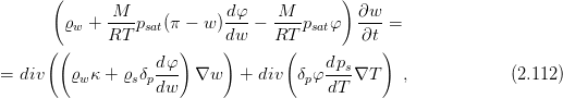
The balance equations

( ) ( ) H (C - C )∂(wCf--)+ ∂Cb-+ ∂Cc-= ∂-- wD ∂Cf- + -∂- C κ ∂w- , (2.108 ) f,sat f ∂t ∂t ∂t ∂x ∂x ∂x f ∂x

( ) ( ) ∂w- ∂-- ∂w- -∂- -δ-∂pv- ∂t = ∂x κ ∂x + ∂x ϱ ∂x , (2.109 ) x

∂Cc ∂ ----= H (Cf - Cf,sat)---(w(Cf - Cf,sat)) , (2.110 ) ∂t ∂t

∂T ∂ ( ∂T ) ∂ ( ∂p ) ϱc ---= --- λ--- + --- Lvδ---v . (2.111 ) ∂t ∂x ∂x ∂x ∂x

The balance equations modified with respect to computer implementation. The balance equation for moisture (mass)

( ) -M-- dφ- -M-- ∂w- ϱw + RT psat(π - w )dw - RT psatφ ∂t = (( ) ) ( ) = div ϱ κ + ϱ δ d-φ ∇w + div δ φ dps∇T , (2.112 ) w s pdw p dT

the balance equation for salt

( ) C H (C - C ) ∂w-+ wH (C - C ) + ∂Cb- ∂Cf- + ∂Cc- = f f,sat f ∂t f,sat f ∂Cf ∂t ∂t = div(wD ∇C ) + div(C κ ∇w ) , (2.113 ) f f

the balance equation for salt

∂Cc ∂ ----= H (Cf - Cf,sat)---(w(Cf - Cf,sat)) , (2.114 ) ∂t ∂t

the balance equation for heat

( ) ( ( ) ) ∂H--∂T- dφ- dps- ∂T ∂t = div Lvδppsatdw ∇w + div λ + Lv δpdT ∇T . (2.115 )

2.3.1.2 Matrix notation

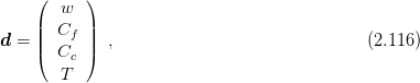
The vector of physical quantities

( ) w || Cf || d = |( |) , (2.116 ) Cc T

the vector of gradients

( [w]) | g[f]| g = || g || , (2.117 ) ( g[c]) g[T]

the vector of flux densities

( ) q[w] || q[f]|| q = |( q[c]|) , (2.118 ) [T] q

the conductivity matrix of material

( ) D [ww ] D [wf] D [wc] D [wT ] || D [fw ] D [ff] D [fc] D [fT] || D = |( [cw] [cf] [cc] [cT] |) , (2.119 ) D [T w] D [Tf] D [Tc] D [TT ] D D D D

the capacity matrix of material

( [ww ] [wf] [wc] [wT]) | H [fw ] H [ff] H [fc] H [fT]| H = || H H H H || . (2.120 ) ( H [cw] H [cf] H [cc] H [cT]) H [T w] H [Tf] H [Tc] H [TT]

The balance eqautions with previous notation

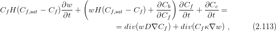
[ww]∂w- [ww] [w] [wT ] [T] H ∂t = div (D g + div(D g ) , (2.121 ) ∂w ∂Cf ∂Cc H [fw]--- + H [ff]---- + H [fc]---- = div (D [fw]gw ]) + div(D [ff]g[f]) , (2.122 ) ∂t ∂t ∂t H [cw]∂w-+ H [cf]∂Cf- + H [cc]∂Cc- = 0 , (2.123 ) ∂t ∂t ∂t [TT]∂T [Tw] [w ] [TT ][T] H ∂t- = div (D g ) + div(D g ) . (2.124 )

The components of capacity matrix of material

[ww] M--- dφ- M--- H = ϱw + RT psat(π - w )dw - RT psatφ , (2.125 ) [wf] H = 0 , (2.126 ) H [wc] = 0 , (2.127 ) H [wT] = 0 , (2.128 )

[fw] H = Cf H (Cf,sat - Cf) , (2.129 ) [ff] ∂Cb- H = wH (Cf,sat - Cf) + ∂C , (2.130 ) f H [fc] = 1 , (2.131 ) H [fT] = 0 , (2.132 )

[cw] H = - (Cf - Cf,sat)H (Cf - Cf,sat) , (2.133 ) H [cf] = - wH (Cf - Cf,sat) , (2.134 ) [cc] H = 1 , (2.135 ) H [cT] = 0 , (2.136 )

[Tw] H = 0 , (2.137 ) H [Tf] = 0 , (2.138 ) [Tc] H = 0 , (2.139 ) [TT] ∂H-- H = ∂T , (2.140 )

the components of conductivity matrix of material

[ww ] dφ D = ϱwκ + ϱsδp dw-, (2.141 ) [wf] D = 0 , (2.142 ) D [wc] = 0 , (2.143 ) dp D [wT ] = δpφ --s-, (2.144 ) dT

D [fw ] = Cfκ , (2.145 ) [ff] D = wD , (2.146 ) D [fc] = 0 , (2.147 ) D [fT ] = 0 , (2.148 )

D [cw] = 0 , (2.149 ) [cf] D = 0 , (2.150 ) D [cc] = 0 , (2.151 ) [cT] D = 0 , (2.152 )

D [T w] = k δ p dφ-, (2.153 ) v p satdw D [Tf] = 0 , (2.154 ) [Tc] D = 0 , (2.155 ) [T T] dps D = λ + Lvδp dT--, (2.156 )

2.3.1.3 Discretization

neznámé veličiny

[w] [w] w = N d (2.157 ) Cf = N [f]d[f] (2.158 ) [c] [c] Cc = N d (2.159 ) T = N [T]d[T] (2.160 )

testovací funkce (jsou aproximovány stejně jako neznámé)

[w ] [w] [w] η = N b (2.161 ) η[f] = N [f]b[f] (2.162 ) η[c] = N [c]b[c] (2.163 ) [T] η[T ] = N [T]b (2.164 )

gradienty

g[w] = B [w ]d [w] (2.165 ) [f] [f] [f] g = B d (2.166 ) g [c] = B [c]d[c] (2.167 ) [T] [T ][T] g = B d (2.168 ) (2.169 )

[ww] [w] [ww] [w] [wT] [T] C ˙d + K d + K d = 0 (2.170 ) [fw ]˙[w] [ff]˙[f] [fc]˙[c] [fw] [w ] [ff] [f] C d + C d + C d + K d + K d = 0 (2.171 ) C [cw]˙d[w] + C [cf]˙d[f] + C [cc]d˙[c] = 0 (2.172 ) [T] C [TT]˙d + K [Tw]d[w] + K [TT]d[T] = 0 (2.173 )

( ) ( [w] ) ( ) ( ) C [ww] 0 0 0 | d˙ | K [ww] 0 0 K [wT] d [w] ( 0 ) || C [fw] C [ff] C [fc] 0 || || d˙[f] || || K [fw] K [ff] 0 0 || || d [f] || | 0 | || [cw] [cf] [cc] || || [c] || + || || || [c] || = || ||(2..174 ) ( C C C 0 ) |( d˙ |) ( 0 0 0 0 ) ( d ) ( 0 ) 0 0 0 C [TT] d˙[T] K [Tw] 0 0 K [TT] d [T] 0

Chapter 3
Time integration methods

Parabolic problems after space discretization lead to systems of ordinary differential equations in the form

dd (t) C ------+ Kd (t) = f (t) , (3.1) dt

where d(t) is the vector of nodal unknowns and f(t) is the vector of given right hand side. In the case of transport processes, f(t) denotes the prescribed fluxes, K is the conductivity matrix and C is the capacity matrix.

3.1 Generalized Trapezoidal Method

The vector of nodal values d evaluated at time instant i + 1 is assumed in the form

di+1 = di + Δtvi+ α , (3.2)

where the vector v_i+α has form

vi+α = (1 - α )vi + αvi+1 . (3.3)

The vector v contains time derivatives of unknown nodal variables, i.e. time derivatives of the vector d. Substitution of expressions (3.2) and (3.3) to the equation (3.1) results in

(C + Δt αK ) vi+1 = fi+1 - K (di + Δt (1 - α)vi) . (3.4)

This formulation is suitable because explicit or implicit computational scheme can be set by parameter α. Advantage of the explicit algorithm is based on possible efficient solution of the system of equations because parameter α can be equal to zero and capacity matrix C can be diagonal. Therefore the solution of the system is extremely easy. The disadvantage of such method is its conditional stability. It means, that the time step must satisfy stability condition what usually leads to very short time step.

In order to abbreviate notation, predictor is defined in the form

d˜i+1 = di + (1 - α )Δtvi (3.5)

The discretized system (3.4) can be therefore rewritten into new form

˜ (C + Δt αK )vi+1 = f i+1 - K di+1 . (3.6)

Either from (3.4) or from (3.6), the vector v_i+1 is obtained and the vector of nodal values at time instant i + 1 has the form

˜ di+1 = di+1 + α Δtvi+1 (3.7)

In the case αΔt≠0, the vector v_i+1 can be expressed from (3.7) in the form

-1---( ˜ ) vi+1 = αΔt di+1 - di+1 (3.8)

which can be substituted to (3.6). After algebraic manipulation, new system of algebraic equations has the form

( 1 ) 1 ----C + K di+1 = f i+1 + -----C ˜di+1 . (3.9) αΔt α Δt

Equation (3.9) is suitable especially for non-linear problems because the nodal values are obtained directly from the system of equations. In the case of (3.6), the time derivatives are obtained and the nodal values have to be computed from (3.7).


Initial vectors		d₀,v₀
(defined by initial conditions)


do until		i ≤ n
		(n is the number of time steps)

predictor		_i+1 = d_i + (1 - α)Δtv_i

right hand side vector		y_i+1 = f_i+1 -K_i+1

matrix of the system		A = C + αΔtK

solution of the system		v_i+1 = A^-1y_i+1

new approximation		d_i+1 = _i+1 + αΔtv_i+1

Table 3.1: v-version of the generalized trapezoidal method.


Initial vectors		d₀,v₀
(defined by initial conditions)


do until		i ≤ n
		(n is the number of time steps)

predictor		_i+1 = d_i + (1 - α)Δtv_i

right hand side vector		y_i+1 = αΔtf_i+1 + C_i+1

matrix of the system		A = C + αΔtK

solution of the system		d_i+1 = A^-1y_i+1

new approximation		v_i+1 =

Table 3.2: d-version of the generalized trapezoidal method.

Contents

List of Tables

Chapter 1Heat transport

1.1 Non-stationary heat transport

Chapter 2Coupled transport of several physical quantities

2.1 General scheme of coupled transport of several physical quantities

2.2 Coupled heat and moisture transport

2.2.1 Künzel model

2.2.1.1 Theoretical description

2.2.1.2 Matrix notation

2.2.1.3 Discretization

2.3 Coupled heat, moisture and salt transport

2.3.1 Černý model

2.3.1.1 Theoretical description

2.3.1.2 Matrix notation

2.3.1.3 Discretization

Chapter 3Time integration methods

3.1 Generalized Trapezoidal Method

Chapter 1
Heat transport

Chapter 2
Coupled transport of several physical quantities

Chapter 3
Time integration methods