
This chapter introduces the notation and terminology used in the manual.
The C programming language contains several data types but only three of them are used in the SIFEL code. The data types are long, double, char. Typical example is the following one
long i;
long is the data type, i is a variable of the type long.
The C++ enables to define additional data types. The SIFEL code uses the data type class. Example of the class is the following
class matrix
{
long m, n;
double *a;
read(FILE *in);
};
matrix mat;
matrix is the data type of class, m, n, a are the attributes (data members, class attributes) of the class matrix, the class matrix contains the member function (method) read(...), mat is an object (instance) of the class matrix.
Another example
class probdesc
{
probtype tp;
};
probdesc Mp;
Mp.tp = linear_statics;
probtype is an enumeration data type, tp is the attribute (data member, class attribute) of the class probdesc, tp is of the type probtype, linear_statics is an enumerator (identifier) from the enumeration probtype.
There are many variables which are described by a function or table. For such description, the class gfunct is implemented. The type of the function is stored in the attribute tfunc and the appropriate keyword is funct_type. The values of the attribute tfunc are summarized in Table 2.1.
| attribute | enumerator | description |
| tfunc = 0 | stat | constant value |
| tfunc = 1 | pars | parser |
| tfunc = 2 | tab | the relationship is described by a table |
If the constant value is selected, the value is stored in the attribute f with the keyword const_val.
If the table is selected, the type of interpolation in the table is read and stored to the attribute itype of the class tablefunct. The keyword for the type of interpolation is approx_type. The values of the attribute itype are summarized in Table 2.2.
| attribute | enumerator | description |
| itype = 1 | piecewiselin | piecewise linear interpolation |
| itype = 2 | piecewiseconst | piecewise constant interpolation |
| itype = 3 | lagrange | Lagrange interpolation |
The number of rows in the table is read and stored in the attribute asize with the keyword ntab_items. After that, asize couples of table entries are read.
Example without keywords
| 0 | # the type of general function - the constant value |
| 234.5 | # the constant value |
Example with keywords
| funct_type stat | # the type of general function - the constant value |
| const_val 234.5 | # the constant value |
Example without keywords
| 2 | # the type of general function - the table |
| 1 | # piecewise linear interpolation |
| 3 | # the number of rows in the table |
| 0.0 234.5 | # first row |
| 10.0 456.32 | # second row |
| 200.0 213.56 | # third row |
Example with keywords
| funct_type tab | # the type of general function - the table |
| approx_type piecewiselin | # piecewise linear interpolation |
| ntab_items 3 | # the number of rows in the table |
| 0.0 234.5 | # first row |
| 10.0 456.32 | # second row |
| 200.0 213.56 | # third row |
Several types of matrix storage are available. The type of storage is located in the attribute ts of the class gmatrix.
| attribute | enumerator | description |
| ts = 0 | without_matrix | matrix is not stored |
| ts = 1 | dense_matrix | all matrix entries are stored row-wise |
| ts = 2 | skyline_matrix | skyline format |
| ts = 3 | double_skyline | double skyline format |
| ts = 10 | compressed_rows | compressed rows |
| ts = 11 | symm_comp_rows | symmetric compressed rows |
| ts = 40 | element_matrices | matrix is not stored, all element |
| matrices are stored consequently | ||
| ts = 140 | spdirect_stor_scr | storage for the sparse direct solver |
| based on symmetric compressed rows | ||
| ts = 141 | spdirect_stor_cr | storage for the sparse direct solver |
| based on compressed rows | ||
| 2 | # the matrix is stored in the skyline storage scheme |
Type of solver of linear algebraic equations is read and stored in the class slesolv to the attribute tlinsol. The values of the attribute tlinsol are summarized in Table 2.4. The keyword for the type of solver is typelinsol.
| attribute | enumerator | description |
| tlinsol = 1 | gauss_elim | Gaussian elimination |
| tlinsol = 2 | ldl | LDLT factorization |
| tlinsol = 3 | lu | LU factorization |
| tlinsol = 4 | ll | LLT factorization |
| tlinsol = 20 | cg | conjugate gradient method |
| tlinsol = 30 | bicg | bi-conjugate gradient method |
| tlinsol = 140 | spdirldl | sparse direct solver based on the LDLT factorization |
| tlinsol = 141 | spdirlu | sparse direct solver based on the LU factorization |
If a direct method is selected, no additional information is needed. If an iterative method is selected, the number of iterations ni (keyword number_of_iterations) and the required norm of residual err (keyword error_of_computation) are required.
The class slesolv contains an object prec of the class precond which is used for reading and storage of data about preconditioners. If an iterative method is selected, the type of preconditioner pt is read. The values of the attribute pt are summarized in Table 2.5.
| attribute | enumerator | description |
| pt = 0 | noprecond | no preconditioner |
| pt = 1 | diagprec | diagonal (Jacobi) preconditioner |
| pt = 5 | ssorprec | SSOR preconditioner |
| pt = 10 | incomdec | preconditioner based on incomplete factorization |
| pt = 101 | boss | BOSS preconditioner |
SSOR preconditioner requires parameter ω stored in the attribute ssoromega and the incompleted factorization requires the threshold for off-diagonal matrix entries rejection which is stored in incompltresh.
Example without keywords
| 2 | # LDL factorization |
Example with keywords
| typelinsol ldl | # LDL factorization |
Example without keywords
| 3 | # LU factorization |
Example with keywords
| typelinsol lu | # LU factorization |
Example without keywords
| 20 | # the conjugate gradient method |
| 400 | # the maximum number of iterations |
| 1.0e-6 | # required norm of residual |
| 0 | # no preconditioner is required |
Example with keywords
| typelinsol cg | # the conjugate gradient method |
| number_of_iterations 400 | # the maximum number of iterations |
| error_of_computation 1.0e-6 | # required norm of residual |
| 0 | # no preconditioner is required |
Example without keywords
| 20 | # the conjugate gradient method |
| 400 | # the maximum number of iterations |
| 1.0e-6 | # required norm of residual |
| 10 | # preconditioner based on incomplete factorization |
| 1.0e-2 | # threshold for off-diagonal entries rejection |
Type of solver of non-linear algebraic equations is read and stored in the class nonlinman to the attribute tnlinsol. The keyword for the type of solver of non-linear algebraic equations is type_of_nonlin_solver. The values of the attribute tnlinsol are summarized in Table 2.6.
| attribute | enumerator | description |
| tnlinsol = 1 | arcl | arc-length method |
| tnlinsol = 2 | newton | the Newton-Raphson method |
After the type of solver of non-linear algebraic equations, the type of the stiffness matrix is read and stored into the attribute stmat described by the keyword stiffmat_type. The attribute stmat has the values summarized in Table 2.7.
| attribute | enumerator | description |
| stmat = 1 | initial_stiff | the initial stiffness matrix |
| stmat = 2 | tangent_stiff | the tangent stiffness matrix |
If the arc-length method is selected, the following parameters have to be defined:
| keyword | abbreviation | description |
| lambda_determination | dlam | type of λ determination |
| al_num_steps | nial | the number of increment |
| al_num_iter | niilal | the number of iterations within increment |
| al_error | erral | required norm of residual |
| al_init_length | dlal | the initial length of the arc |
| al_min_length | dlminal | the minimum lenght of arc |
| al_max_length | dlmaxal | the maximum lenght of arc |
| al_psi | psial | the parameter ψ |
| al_displ_contr_type | displnorm | the type of displacement norm |
Determination of λ described by the attribute has the following possibilities
| attribute | enumerator | description |
| detlambda=0 | nodetermination | the determination is not defined |
| detlambda=1 | minvalue | the minimum value is used |
| detlambda=2 | maxvalue | the maximum value is used |
| detlambda=3 | minangle | the minimum angle is used |
| detlambda=4 | linearizedmeth | linearized arc-length method is used |
| detlambda=5 | fullmethod | the full method is used |
Displacement norm described by the attribute displnorm and by the keyword al_displ_contr_type has the following possibilities
| attribute | enumerator | description |
| displnorm=1 | alldofs | all degrees of freedom are used |
| displnorm=2 | seldofs | selected degrees of freedom are used |
| displnorm=3 | seldofscoord | |
| displnorm=6 | selecnodes | DOFs defined in selected nodes are used |
| displnorm=8 | nodesdistincr | norm of distance increment of selected nodes |
If the selected degrees of freedom are selected, the number of selected DOFs has to be stored in the attribute nsdofal described by the keyword num_sel_dofs. Then, a list of selected node numbers and DOFs follows.
If the selected nodes are used, the number of nodes is stored in the attribute num_sel_nodes. Then, a list of the selected node numbers follows.
If the Newton-Raphson method is selected, the following parameters have to be defined:
| keyword | enumerator | description |
| nr_num_steps | ninr | the number of increments |
| nr_num_iter | niilnr | the number of iterations within increments |
| nr_error | errnr | required norm of residual |
| nr_init_incr | incrnr | the intial increment |
| nr_minincr | minincrnr | the minimum increment |
| nr_maxincr | maxincrnr | the maximum increment |
Example without keywords
| 1 | # the arc-length method is used |
| 1 | # the initial stiffness matrix is used |
| 1 | # determination of lambda (the minimum values is used) |
| 300 | # the number of increments |
| 30 | # the number of iterations within increment |
| 1.0e-04 | # the required norm of residual |
| 1.0e-01 | # the initial lenght of arc |
| 1.0e-08 | # the minimum length of arc |
| 1.0e+03 | # the maximum length of arc |
| 0 | # the parameter psi |
| 1 | # the type of displacement norm (all DOFs in this case) |
Example with keywords
| type_of_nonlin_solver arcl | # the arc-length method is used |
| stiffmat_type initial_stiff | # the initial stiffness matrix is used |
| lambda_determination minvalue | # the minimum value is used |
| al_num_steps 300 | # the number of increments |
| al_num_iter 30 | # the number of iterations within increment |
| al_error 1.0e-04 | # the required norm of residual |
| al_init_length 1.0e-01 | # the initial lenght of arc |
| al_min_length 1.0e-08 | # the minimum length of arc |
| al_max_length 1.0e+03 | # the maximum length of arc |
| al_psi 0 | # the parameter psi |
| al_displ_contr_type alldofs | # the type of displacement norm |
| # (all DOFs in this case) | |
Example without keywords
| 1 | # the arc-length method is used |
| 2 | # the tangent stiffness matrix is used |
| 1 | # determination of lambda (the minimum values is used) |
| 300 | # the number of increments |
| 30 | # the number of iterations within increment |
| 1.0e-04 | # the required norm of residual |
| 1.0e-01 | # the initial lenght of arc |
| 1.0e-08 | # the minimum length of arc |
| 1.0e+03 | # the maximum length of arc |
| 0 | # the parameter psi |
| 2 | # the type of displacement norm (selected DOFs in this case) |
| 4 | # the number of selected DOFs |
| 12 1 | # first DOF in the 12th node |
| 23 1 | # first DOF in the 23rd node |
| 45 2 | # second DOF in the 45th node |
| 78 3 | # third DOF in the 78th node |
Example with keywords
| type_of_nonlin_solver arcl | # the arc-length method is used |
| stiffmat_type initial_stiff | # the initial stiffness matrix is used |
| lambda_determination minvalue | # the minimum value is used |
| al_num_steps 300 | # the number of increments |
| al_num_iter 30 | # the number of iterations within increment |
| al_error 1.0e-04 | # the required norm of residual |
| al_init_length 1.0e-01 | # the initial lenght of arc |
| al_min_length 1.0e-08 | # the minimum length of arc |
| al_max_length 1.0e+03 | # the maximum length of arc |
| al_psi 0 | # the parameter psi |
| al_displ_contr_type seldofs | # selected DOFs |
| num_sel_dofs 4 | # the number of selected DOFs |
| 12 1 | # first DOF in the 12th node |
| 23 1 | # first DOF in the 23rd node |
| 45 2 | # second DOF in the 45th node |
| 78 3 | # third DOF in the 78th node |
Example without keywords
| 2 | # the Newton-Raphson method is used |
| 1 | # the initial stiffness matrix is used |
| 500 | # the number of increments |
| 40 | # the number of iterations within increment |
| 1.0e-04 | # the required norm of residual |
| 1.0e-01 | # the initial increment |
| 1.0e-08 | # the minimum increment |
| 1.0e+03 | # the maximum increment |
Example with keywords
| tnlinsol newton | # the Newton-Raphson method is used |
| stiffmat_type initial_stiff | # the initial stiffness matrix is used |
| nr_num_steps 500 | # the number of increments |
| nr_num_iter 40 | # the number of iterations within increment |
| nr_error 1.0e-04 | # the required norm of residual |
| nr_init_incr 1.0e-01 | # the initial increment |
| nr_minincr 1.0e-08 | # the minimum increment |
| nr_maxincr 1.0e+03 | # the maximum increment |
Type of time controller is read and stored in the class timecontr to the attribute tct. The values of the attribute tct are summarized in Table 2.8. The keyword for the type of time controller is time_contr_type.
| attribute | enumerator | description |
| tct = 0 | fixed | the time step is constant |
| tct = 1 | adaptive | the time step is changed |
| tct = 2 | adaptivemin | the time step is only reduced |
| tct = 3 | adaptivemax | the time step is only increased |
Starting time is stored in the attribute start_time with the keyword start_time. End time is stored in the attribute end_time with the keyword end_time. The important times are time instants when the solver certainly computes the response without respect to the time steps. The number of important times is stored in the attribute nit and the keyword is num_imp_times.
The time step is governed by an instance timefun of the class gfunct. Setting of the instances of the class gfunct are described in Section 2.1.
If the type of time controller is adaptive, the minimum time step stored in the attribute dtmin with the keyword dtmin and the maximum time step stored in the attribute dtmax with the keyword dtmax are required. If the type of time controller is adaptivemin, the minimum time step stored in the attribute dtmin with the keyword dtmin is required. If the type of time controller is adaptivemax, the maximum time step stored in the attribute dtmax with the keyword dtmax is required.
Example without keywords
| 0 | # the type of time controller - fixed |
| 0.0 | # the starting time |
| 123.0 | # the end time |
| 0 | # the number of important times |
| 0 | # the type of general function governing the time step |
| # the constant value | |
| 2.5 | # the time step |
Example with keywords
| time_contr_type fixed | # the type of time controller - fixed |
| 0.0 | # the starting time |
| 123.0 | # the end time |
| 0 | # the number of important times |
| funct_type stat | # the type of general function - the constant value |
| const_val 2.5 | # the time step |
Example without keywords
| 0 | # the type of time controller - fixed |
| 0.0 | # the starting time |
| 123.0 | # the end time |
| 0 | # the number of important times |
| 2 | # the type of general function governing the time step |
| # the table | |
| 1 | # piecewise linear interpolation |
| 3 | # the number of rows in the table |
| 0.0 2.5 | # first row |
| 10.0 5.0 | # second row |
| 200.0 20.0 | # third row |
Example with keywords
| time_contr_type fixed | # the type of time controller - fixed |
| 0.0 | # the starting time |
| 123.0 | # the end time |
| 0 | # the number of important times |
| funct_type tab | # the type of general function - the table |
| approx_type piecewiselin | # piecewise linear interpolation |
| ntab_items 3 | # the number of rows in the table |
| 3 | # the number of rows in the table |
| 0.0 2.5 | # first row |
| 10.0 5.0 | # second row |
| 200.0 20.0 | # third row |
Example without keywords
| 1 | # the type of time controller - adaptive |
| 0.0 | # the starting time |
| 123.0 | # the end time |
| 0 | # the number of important times |
| 0 | # the type of general function governing the time step |
| # the constant value | |
| 2.5 | # the time step |
| 1.0e-4 | # the minimum time step |
| 1.0e2 | # the maximum time step |
Example with keywords
| time_contr_type adaptive | # the type of time controller - adaptive |
| 0.0 | # the starting time |
| 123.0 | # the end time |
| 0 | # the number of important times |
| funct_type stat | # the type of general function - the constant value |
| const_val 2.5 | # the time step |
| dtmin 1.0e-4 | # the minimum time step |
| dtmax 1.0e2 | # the maximum time step |
Type of node renumbering is read and stored in the class gtopology to the attribute nodren. The values of the attribute nodren are summarized in Table 2.9. The keyword for the type of node renumbering is noderenumber.
| attribute | enumerator | description |
| nodren = 0 | no_renumbering | no renumbering |
| nodren = 1 | cuthill_mckee | Cuthill-McKey renumbering |
| nodren = 2 | rev_cuthill_mckee | reverse Cuthill-McKey renumbering |
| nodren = 3 | sloan | Sloan renumbering |
Example without keywords
| 0 | # nodes are not renumbered |
Example with keywords
| noderenumber no_renumbering | # nodes are not renumbered |
There are three attributes devoted to the strain computation. The attribute straincomp with the keyword straincomp indicates whether the strains are computed and stored. The attribute strainpos with the keyword strainposdefines the position where the strains are computed. The attribute strainaver with the keyword strainaver defines whether the strains are averaged. The strains are averaged only in the case that they are required in nodes where contributions from all adjacent finite elements are added. Values of all attributes are summarized in Tables 2.10, 2.11 and 2.12.
| attribute | description |
| straincomp = 0 | strains are not computed and stored |
| straincomp = 1 | strains are computed and stored |
| attribute | description |
| strainpos = 1 | strains are computed and stored in integration points |
| strainpos = 2 | strains are computed in integration points and stored in nodes |
| strainpos = 3 | strains are computed and stored in nodes |
| attribute | description |
| strainaver = 0 | strains are not averaged |
| strainaver = 1 | strains are averaged in nodes |
Example without keywords
| 0 | # strains are not computed and stored |
Example with keywords
| straincomp 0 | # strains are not computed and stored |
Example without keywords
| 1 | # strains are computed and stored |
| 3 | # strains are computed in nodes |
| 1 | # the final strains are average values of strains from adjacent elements |
There are three attributes devoted to the stress computation. The attribute stresscomp with the keyword stresscomp indicates whether the stresses are computed and stored. The attribute stresspos with the keyword stresspos defines the position where the stresses are required. Stresses can be computed only in integration points because of definition of material models. The attribute stressaver with the keyword stressaver defines whether the stresses are averaged. The stresses are averaged only in the case that they are required in nodes where contributions from all adjacent finite elements are added. Values of all attributes are summarized in Tables 2.13, 2.14 and 2.15.
| attribute | description |
| stresscomp = 0 | stresses are not computed and stored |
| stresscomp = 1 | stresses are computed and stored |
| attribute | description |
| stresspos = 1 | stresses are computed and stored in integration points |
| stresspos = 2 | stresses are computed in integration points and stored in nodes |
| attribute | description |
| stressaver = 0 | stresses are not averaged |
| stressaver = 1 | stresses are averaged in nodes |
Example without keywords
| 0 | # stresses are not computed and stored |
Example without keywords
| 1 | # stresses are computed and stored |
| 2 | # stresses are computed in nodes |
| 1 | # the final stresses are average values of stresses from adjacent elements |
There are three attributes devoted to the computation of internal variables. The attribute othercomp with the keyword othercomp indicates whether the internal variables are computed and stored. The attribute otherpos with the keyword otherpos defines the position where the internal variables are required. The internal variables can be computed only in integration points where the material models are defined. The attribute othernaver with the keyword otheraver defines whether the internal variables are averaged. The internal variables are averaged only in the case that they are required in nodes where contributions from all adjacent finite elements are added. Values of all attributes are summarized in Tables 2.16, 2.17 and 2.18.
| attribute | description |
| othercomp = 0 | internal variables are not computed and stored |
| othercomp = 1 | internal variables are computed and stored |
| attribute | description |
| otherpos = 1 | internal variables are computed and stored in integration points |
| otherpos = 2 | internal variables computed in integration points and stored in nodes |
| attribute | description |
| otheraver = 0 | internal variables are not averaged |
| otheraver = 1 | internal variables are averaged in nodes |
Example without keywords
| 0 | # internal variables are not computed and stored |
Example without keywords
| 1 | # internal variables are computed and stored |
| 2 | # internal variables are computed in nodes |
| 1 | # the final internal variables are average values of |
| # internal variables from adjacent elements | |
There are three attributes devoted to the gradient computation. The attribute gradcomp with the keyword gradcomp indicates whether the gradients are computed and stored. The attribute gradpos with the keyword gradpos defines the position where the gradients are required. The attribute gradaver with the keyword gradaver defines whether the gradients are averaged. The gradients are averaged only in the case that they are required in nodes where contributions from all adjacent finite elements are added. Values of all attributes are summarized in Tables 2.19, 2.20 and 2.21.
| attribute | description |
| gradcomp = 0 | gradients are not computed and stored |
| gradcomp = 1 | gradients are computed and stored |
| attribute | description |
| gradpos = 1 | gradients are computed and stored in integration points |
| gradpos = 2 | gradients are computed in integration points and stored in nodes |
| gradpos = 3 | gradients are computed and stored in nodes |
| attribute | description |
| gradaver = 0 | gradients are not averaged |
| gradaver = 1 | gradients are averaged in nodes |
Example without keywords
| 0 | # gradients are not computed and stored |
Example without keywords
| 1 | # gradients are computed and stored |
| 2 | # gradients computed in nodes |
| 1 | # the final gradients are average values of gradients from adjacent elements |
There are three attributes devoted to the flux computation. The attribute fluxcomp with the keyword fluxcomp indicates whether the fluxes are computed and stored. The attribute fluxpos with the keyword fluxpos defines the position where the fluxes are required. Fluxes can be computed only in integration points because of definition of material models. The attribute fluxaver with the keyword fluxaver defines whether the fluxes are averaged. The fluxes are averaged only in the case that they are required in nodes where contributions from all adjacent finite elements are added. Values of all attributes are summarized in Tables 2.22, 2.23 and 2.24.
| attribute | description |
| fluxcomp = 0 | fluxes are not computed and stored |
| fluxcomp = 1 | fluxes are computed and stored |
| attribute | description |
| fluxpos = 1 | fluxes are computed and stored in integration points |
| fluxpos = 2 | fluxes are computed in integration points and stored in nodes |
| attribute | description |
| fluxaver = 0 | fluxes are not averaged |
| fluxaver = 1 | fluxes are averaged in nodes |
Example without keywords
| 0 | # fluxes are not computed and stored |
Example without keywords
| 1 | # fluxes are computed and stored |
| 2 | # fluxes are computed in nodes |
| 1 | # the final fluxes are average values of fluxes from adjacent elements |
For the purposes of the finite element method, the domains solved are described by entities and their “properties” (markers). The entities are vertices, edges, surfaces, regions, patches and shells. The entities are denoted by integer numbers summarized in Table 3.1.
| entity | entity number |
| vertex | 1 |
| edge | 2 |
| surface | 3 |
| region | 4 |
| patch | 5 |
| shell | 6 |
Finite element meshes obtained from mesh generators are summarized in Table 3.2.
| element | the number | the number | the number | element description |
| type | of nodes | of edges | of surfaces | |
| one-dimensional elements | ||||
| 1 | 2 | 1 | 0 | line with linear shape functions |
| 2 | 3 | 1 | 0 | line with quadratic shape functions |
| (there is midside node) | ||||
| two-dimensional elements | ||||
| 3 | 3 | 3 | 1 | triangular element with linear shape functions |
| 4 | 6 | 3 | 1 | triangular element with quadratic shape functions |
| (there are mid-edge nodes) | ||||
| 5 | 4 | 4 | 1 | quadrilateral element with linear shape functions |
| 6 | 8 | 4 | 1 | quadrilateral element with quadratic shape functions |
| (there are mid-edge nodes) | ||||
| three-dimensional elements
| ||||
| 7 | 4 | 6 | 4 | tetrahedral element with linear shape functions |
| 8 | 10 | 6 | 4 | tetrahedral element with quadratic shape functions |
| (there are mid-edge nodes) | ||||
| 9 | 5 | 8 | 5 | pyramid element with linear shape functions |
| 10 | 13 | 8 | 5 | pyramid element with quadratic shape functions |
| (there are mid-edge nodes) | ||||
| 11 | 6 | 9 | 5 | triangular prism element with linear shape functions |
| 12 | 15 | 9 | 5 | triangular prism element with quadratic shape functions |
| (there are mid-edge nodes) | ||||
| 13 | 8 | 12 | 6 | hexahedral elements with linear shape functions |
| 14 | 20 | 12 | 6 | hexahedral elements with quadratic shape functions |
| (there is mid-edge node) | ||||
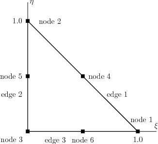
| edge number | node numbers |
| 1 | 1, 2 |
| 2 | 2, 3 |
| 3 | 3, 1 |
| edge number | node numbers |
| 1 | 1, 2, 4 |
| 2 | 2, 3, 5 |
| 3 | 3, 1, 6 |
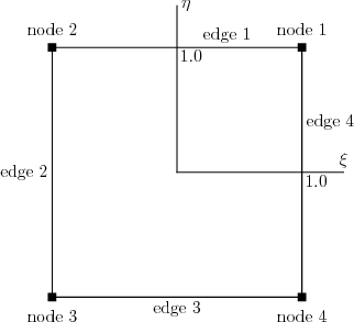
| edge number | node numbers |
| 1 | 1, 2 |
| 2 | 2, 3 |
| 3 | 3, 4 |
| 4 | 4, 1 |
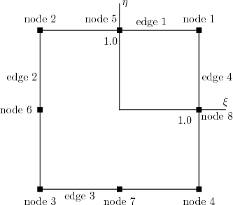
| edge number | node numbers |
| 1 | 1, 2, 5 |
| 2 | 2, 3, 6 |
| 3 | 3, 4, 7 |
| 4 | 4, 1, 8 |
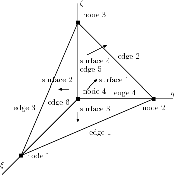
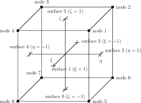
| surface number | node numbers |
| 1 | 1, 4, 8, 5 |
| 2 | 2, 1, 5, 6 |
| 3 | 3, 2, 6, 7 |
| 4 | 4, 3, 7, 8 |
| 5 | 1, 2, 3, 4 |
| 6 | 5, 6, 7, 8 |
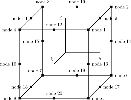 |  |
| surface number | node numbers |
| 1 | 1, 4, 8, 5, 12, 16, 20, 13 |
| 2 | 2, 1, 5, 6, 9, 13, 17, 14 |
| 3 | 3, 2, 6, 7, 10, 14, 18, 15 |
| 4 | 4, 3, 7, 8, 11, 15, 19, 16 |
| 5 | 1, 2, 3, 4, 9, 10, 11, 12 |
| 6 | 5, 6, 7, 8, 17, 18, 19, 20 |
node id, x coordinate, y coordinate, z coordinate, the number of properties (np), np couples of integer numbers, where the first number in every couple is entity type (see Table 3.1) and the second integer denotes property
The block containing elements starts with the number of elements in the mesh. A typical line of element block has the following structure
element id, type of element, element nodes, surface property, edge properties and volume properties
| 16 | |||||||||||
| 1 | 0.00000000000e+00 | 0.00000000000e+00 | 0.0 | 5 | 1 3 | 2 2 | 2 3 | 3 1 | 4 1 | ||
| 2 | 0.00000000000e+00 | 3.33333333333e+00 | 0.0 | 4 | 1 0 | 2 2 | 3 1 | 4 1 | |||
| 3 | 0.00000000000e+00 | 6.66666666667e+00 | 0.0 | 4 | 1 0 | 2 2 | 3 1 | 4 1 | |||
| 4 | 0.00000000000e+00 | 1.00000000000e+01 | 0.0 | 5 | 1 2 | 2 1 | 2 2 | 3 1 | 4 1 | ||
| 5 | 3.33333333333e+00 | 0.00000000000e+00 | 0.0 | 4 | 1 0 | 2 3 | 3 1 | 4 1 | |||
| 6 | 3.33333333333e+00 | 3.33333333333e+00 | 0.0 | 3 | 1 0 | 3 1 | 4 1 | ||||
| 7 | 3.33333333333e+00 | 6.66666666667e+00 | 0.0 | 3 | 1 0 | 3 1 | 4 1 | ||||
| 8 | 3.33333333333e+00 | 1.00000000000e+01 | 0.0 | 4 | 1 0 | 2 1 | 3 1 | 4 1 | |||
| 9 | 6.66666666667e+00 | 0.00000000000e+00 | 0.0 | 4 | 1 0 | 2 3 | 3 1 | 4 1 | |||
| 10 | 6.66666666667e+00 | 3.33333333333e+00 | 0.0 | 3 | 1 0 | 3 1 | 4 1 | ||||
| 11 | 6.66666666667e+00 | 6.66666666667e+00 | 0.0 | 3 | 1 0 | 3 1 | 4 1 | ||||
| 12 | 6.66666666667e+00 | 1.00000000000e+01 | 0.0 | 4 | 1 0 | 2 1 | 3 1 | 4 1 | |||
| 13 | 1.00000000000e+01 | 0.00000000000e+00 | 0.0 | 5 | 1 4 | 2 3 | 2 4 | 3 1 | 4 1 | ||
| 14 | 1.00000000000e+01 | 3.33333333333e+00 | 0.0 | 4 | 1 0 | 2 4 | 3 1 | 4 1 | |||
| 15 | 1.00000000000e+01 | 6.66666666667e+00 | 0.0 | 4 | 1 0 | 2 4 | 3 1 | 4 1 | |||
| 16 | 1.00000000000e+01 | 1.00000000000e+01 | 0.0 | 5 | 1 1 | 2 1 | 2 4 | 3 1 | 4 1 | ||
| 9 | |||||||||||||
| 1 | 5 | 1 | 5 | 6 | 2 | 1 | 3 | 0 | 0 | 2 | 1 | ||
| 2 | 5 | 2 | 6 | 7 | 3 | 1 | 0 | 0 | 0 | 2 | 1 | ||
| 3 | 5 | 3 | 7 | 8 | 4 | 1 | 0 | 0 | 1 | 2 | 1 | ||
| 4 | 5 | 5 | 9 | 10 | 6 | 1 | 3 | 0 | 0 | 0 | 1 | ||
| 5 | 5 | 6 | 10 | 11 | 7 | 1 | 0 | 0 | 0 | 0 | 1 | ||
| 6 | 5 | 7 | 11 | 12 | 8 | 1 | 0 | 0 | 1 | 0 | 1 | ||
| 7 | 5 | 9 | 13 | 14 | 10 | 1 | 3 | 4 | 0 | 0 | 1 | ||
| 8 | 5 | 10 | 14 | 15 | 11 | 1 | 0 | 4 | 0 | 0 | 1 | ||
| 9 | 5 | 11 | 15 | 16 | 12 | 1 | 0 | 4 | 1 | 0 | 1 | ||
In mechanical analyses, a local coordinate system may be suitable. The presence of the local coordinate system is indicated by the attribute transf of the class node. Values of the attribute transf are summarized in Table 3.9.
| attribute | description |
| transf = 0 | no local coordinate system |
| transf = 2 | 2D problem, two basis vectors are required |
| transf = 3 | 3D problem, three basis vectors are required |
| 0 | # no local coordinate system |
| 2 0.6 0.8 -0.8 0.6 | # local coordinate system in 2D |
| 3 0.6 0.8 0.0 -0.8 0.6 0.0 0.0 0.0 1.0 | # local coordinate system in 3D |
Typical line of an input file describing a node is the following
id x y z NDOF crsec locsys
id is node number, x, y and z are coordinates, NDOF is the number of degrees of freedom defined in the node, crsec is description of cross section and locsys describes a local coordinate system in the node. Local coordinate system is used in mechanical problems only, it is not used in transport processes. Definition of cross section is in Section 5.1. Definition of local coordinate system is in Section 3.2.
| 4 | # the number of nodes in mesh |
| 1 0.0 0.0 0.0 2 0 0 | |
| 2 2.0 1.0 0.0 2 0 0 | |
| 3 4.0 2.0 0.0 2 0 0 | |
| 4 6.0 3.0 0.0 2 0 0 | |
| 4 | # the number of nodes in mesh |
| 1 0.0 0.0 0.0 2 0 | |
| 2 2.0 1.0 0.0 2 0 | |
| 3 4.0 2.0 0.0 2 0 | |
| 4 6.0 3.0 0.0 2 0 | |
| 4 | # the number of nodes in mesh |
| 1 0.0 0.0 0.0 2 1 1 0 | |
| 2 2.0 1.0 0.0 2 1 1 0 | |
| 3 4.0 2.0 0.0 2 1 1 0 | |
| 4 6.0 3.0 0.0 2 1 1 0 | |
| 4 | # the number of nodes in mesh |
| 1 0.0 0.0 0.0 3 0 0 | |
| 2 2.0 1.0 0.0 3 0 2 0.6 0.8 -0.8 0.6 | |
| 3 4.0 2.0 0.0 3 0 0 | |
| 4 6.0 3.0 0.0 3 0 0 | |
| 4 | # the number of nodes in mesh |
| 1 0.0 0.0 3.0 3 0 0 | |
| 2 2.0 1.0 2.0 3 0 3 0.6 0.8 0.0 -0.8 0.6 0.0 0.0 0.0 1.0 | |
| 3 4.0 2.0 1.0 3 0 0 | |
| 4 6.0 3.0 0.0 3 0 0 | |
Hanging nodes are nodes which are linearly dependent on other nodes in a mesh. The nodes which the hanging nodes depend on are called tha master nodes. Degrees of freedom of any hanging node are defined by the master nodes. The hanging nodes are therefore indicated by negative value of the attribute ndofn of the class gnode which defines the number of degrees of freedom of the node. The absolute value of the attribute ndofn is equal to the number of master node.
The 132nd node is a hanging node, it is connected to an edge, its master nodes are the nodes 143 and 345, the natural coordinate on the edge is 0.4, 0.0 and 0.0. The edge is indicated by the number 1 after the natural coordinates. The last two zeros indicate the cross section and local coordinate system in the 132-nd node.
| 132 1.4 2.3 3.7 -2 143 345 0.4 0.0 0.0 1 0 0 | # hanging node |
The 132nd node is a hanging node, it is connected to a surface, its master nodes are the nodes 143, 345, 356 and 378, the natural coordinate on the surface are 0.3, 0.8 and 0.0. The surface is indicated by the number 5.
| 132 1.4 2.3 3.7 -4 143 345 356 378 0.3 0.8 0.0 5 0 0 | # hanging node |
The 132nd node is a hanging node, it is connected to a volume, its master nodes are the nodes 143, 345, 356, 378, 412, 456, 478 and 567 the natural coordinate in the volume are 0.5, 0.4 and 0.9.
| 132 1.4 2.3 3.7 -8 143 345 356 378 412 456 478 567 0.5 0.4 0.9 13 0 0 | # hanging node |
List of material parameters
| notation | unit | parameter |
| E | Pa | Young modulus of elasticity |
| G | Pa | shear modulus of elasticity |
| μ | - | Poisson ratio |
| ϱ | kg/m3 | density |
| α | K-1 | coefficient of thermal expansion (thermal extensibility coefficient) |
| λ | J/m/s | coefficient of heat conductivity |
| c | J/kg/K | heat capacity coefficient |
| material | materiál | E GPa | G GPa | ν | ϱ kg/m3 | α 10-6 K-1 | λ J/m/s | c J/kg/K |
| aluminium | hliník | 66 - 68 | 26 - 28 | 0.33 | 2 650 - 2 800 | 20 - 24 | 125 - 229 | 896 - 1 000 |
| asphalt | asfalt | 1 300 | 0.7 | |||||
| bricks | cihly | 8 - 12 | 1 400 - 2 200 | 5 | 0.28 - 1.2 | 900 - 1 100 | ||
| concrete | beton | 15 - 40 | 0.08 - 0.18 | 1 800 - 2 500 | 12 | 1.2 - 1.75 | 850 - 1 200 | |
| conc. cellular | pórobeton | 0.8 - 4 | 400 - 900 | 7 - 8 | 0.12 - 0.35 | 850 | ||
| copper | měd’ | 120 - 130 | 42 - 47 | 0.34 | 8 930 | 17 | 395 | 383 |
| cork | korek | 200-350 | ||||||
| glass | sklo | 70 | 2 400 - 4 700 | 6 - 9 | 0.6 - 1 | |||
| granite | žula | 27 - 51 | 2 600 - 2 900 | 7.89 | 2.9 - 4 | |||
| ice | led | 917 | 50 | 2.2 | ||||
| iron | železo | 7 860 | 12 | 73 | 452 | |||
| paper | papír | 700 - 1 100 | ||||||
| polystyrene | polystyrén | 0.0028 - 0.015 | - | - | 14 - 100 | 50 - 80 | 0.035 - 0.045 | 1 350 |
| PVC | PVC | 2.5 - 3.6 | 1 360 - 1 400 | 80 | 0.15 | 1 000 - 1 100 | ||
| rubber | guma | 1 150 - 1 350 | ||||||
| snow | sníh | 125 - 800 | 0.12 - 1.3 | |||||
| steel | ocel | 210 | 85 | 0.3 | 7 400 - 8 000 | 12 | 50 - 58 | 460 |
| wood | dřevo | 10 - 15 | 0.3 - 0.6 | - | 400 - 1 000 | 3 - 32 | 0.09 - 0.2 | 2 100 - 2 700 |
| wool (glass) | vlna (skelná) | - | - | - | 12 | - | 0.03 - 0.05 | |
Linear elastic isotropic model requires definition of two material parameters: the Young modulus os elasticity E (Pa) and the Poisson ratio μ (-).
Example without keywords
| 1 | # there is single type of material model |
| 1 2 | # first material model is linear elastic isotropic model and there are two instances of such type |
| 1 20.e9 0.1 | # first instance of the elastic model (Young modulus of elasticity, Poisson ratio) |
| 2 30.0e9 0.13 | # second instance of the elastic model (Young modulus of elasticity, Poisson ratio) |
Linear isotropic transport model requires definition of the coefficient of heat conductivity λ (J/m/s). In the case on non-stationary transport, also the heat capacity c (J/kg/K) is required.
Example without keywords
| 1 | # there is single type of material model |
| 100 2 | # first material model is linear isotropic model and there are two instances of such type |
| 1 1.5 | # first instance of the isotropic model (the coefficient of conductivity) |
| 2 1.9 | # second instance of the isotropic model (the coefficient of conductivity) |
Example without keywords
| 1 | # there is single type of material model |
| 100 2 | # first material model is linear isotropic model and there are two instances of such type |
| 1 1.5 900.0 | # first instance of the isotropic model (the coefficient of conductivity, capacity coefficient) |
| 2 1.9 980.0 | # second instance of the isotropic model (the coefficient of conductivity, capacity coefficient) |
2. the bulk density of the sample ρ (kg/m3), 3. porosity 4. water vapour diffusion resistance factor μ, 5. the moisture diffusivity κ (m2/s), 9. specific heat capacity of the building material cs (J/kg/K), 10. thermal conductivity λ (W/m/K)
w is the volumetric moisture content (m3/m3), T is the temperature (K), κ is the moisture diffusivity (m2/s), δ is the water vapour diffusion permeability (s), ρ w is the density of water (kg/m3), p v is the partial pressure of water vapour (Pa), c is the specific heat capacity (J/kg/K), λ is the thermal conductivity (W/m/K) and Lv is the latent heat of evaporation of water (J/kg).
list of material parameters used in the model: position CORD: 2 - density 3 - porosity 4 - water vapour diffusion resistance factor 5 - moisture diffusivity 6 - sorption isoterm 7 - saturated moisture 8 - none 9 - specific heat capacity 10 - thermal conductivity 11 - 13 - none 14 Dcoef 15 - binding isotherm 16 - cfmax 17 ws 18 - none 19 - kunzeltype
| attribute | enumerator | description |
| crst=0 | nocrosssection | no cross section |
| crst=1 | csbar2d | cross section for bar element |
| crst=2 | csbeam2d | cross section for 2D beams |
| crst=4 | csbeam3d | cross section for 3D beams |
| crst=10 | csplanestr | cross section for plane strain and plane stress problems |
| crst=20 | cs3dprob | cross section for three-dimensional problems |
If the cross section is not defined in connection with a quantity (node or element), 0 or nocrosssection is put into appropriate position. On the other hand, if the cross section is defined, two values are required. The first is the type of the cross section and the second is the id of the appropriate instance of the cross section type.
Example without keywords
| 0 | # the cross section is not defined on element or node |
Example without keywords
| 2 | # the cross section for 2D beam is defined |
| 3 | # third instance of all 2D beam cross sections is selected |
All cross sections are summarized in one list.
Example without keywords
| 2 | # there are two types of cross sections |
| 1 3 | # first cross section type is for 2D bar elements and there are 3 instances of such type |
| 1 0.03 | # first instance of the bar cross section |
| 2 0.02 | # second instance of the bar cross section |
| 3 0.06 | # third instance of the bar cross section |
| 2 2 | # second cross section type is for 2D beam elements and there are 2 instances of such type |
| 1 0.04 0.0005 0.8333 | # first instance of the beam cross section |
| 2 0.05 0.0004 0.8333 | # second instance of the beam cross section |
The class is used in outdriverm and outdrivert classes (MEFEL, TRFEL) and it contains the selection of variety items such as load cases, time steps, nodes, elements, particular quantities defined at nodes or elements, etc. Depending on the selected items or quantities, integer indeces or real numbers are used for the selection. Type of sel is given by the st attribute whose values are defined by enumeration seltype (see galias.h) which is described in the following table.
| attribute | enumerator | description |
| st = 0 | sel_no | nothing is selected |
| st = 1 | sel_all | all values/indeces are selected |
| st = 2 | sel_range | selection by ranges of indeces |
| st = 3 | sel_list | selection by list of individual indeces |
| st = 4 | sel_period | selection by constant period |
| (each n-th index is selected) | ||
| st = 5 | sel_realrange | selection by range of real values |
| st = 6 | sel_reallist | selection by list of real values |
| st = 7 | sel_mtx | selection of all components of a tensorial |
| quantity for GiD | ||
| st = 8 | sel_range_mtx | selection of all components of a tensorial quantity |
| for GiD by range of indeces, the quantity | ||
| is stored in larger array (e.g. eqother) | ||
| st = 9 | sel_range_vec | selection of a vector quantity for GiD |
| by range of indeces - the quantity | ||
| is stored inside larger array (e.g. eqother) | ||
| st = 10 | sel_realperiod | option used for selection of time steps with |
| real period r | ||
| st = 11 | sel_impvalues | option used for selection of time steps |
| according to important times defined in | ||
| time controller (class timecontr) | ||
The class sel has also attribute n which represents the number of selected ranges or items depending on the type of selection (st attribute).
| st = 0 | n = 0 |
| st = 1 | n = 1 |
| st = 2 | n = number of selected ranges |
| st = 3 | n = number of list items |
| st = 4 | n = 1 |
| st = 5 | n = number of selected real ranges |
| st = 6 | n = number of real items in the list |
| st = 7 | n = 1 |
| st = 8 | n = 1 |
| st = 9 | n = 1 |
| st = 10 | n = number is calculated from the time |
| interval length and given period | |
| st = 11 | n = 1 |
The class sel was designed for the selection of output data and there is often required the output of different quantities for given selection of elements or nodes. The typical case represents output of selected internal variables stored in the eqother array on integration points of elements. If the problem domain is heterogeneous and different material models are used then the order of internal variables is not the same for all integration points and consequently, the selection of required internal variables differs on particular elements. This case can be solved by using of conjugated selections where the main selection is connected with required elements/nodes and conjugated selection is connected with the required internal variables. The number of conjugated selections is given by the number of items in the main selection, i.e., attribute n of main selection is the number of conjugated selections.
In the cases of stress or strain selection, the conjugated selection consists of main selection of nodes/elements, conjugated selections of stress/strain components and conjugated flags for output of principal stresses/strains. Similarly, the number of conjugated selections and conjugated flags is given by the number of items in the main selection (attribute n).
This section describes basic selections used for selection of list of integer identifiers or indeces (ids), e.g. nodes, elements, load cases, strain components, time steps, etc.
Example without keywords
| 0 | # type of selection = no selection or empty list |
Example with keywords
| sel_no | # type of selection = no selection or empty list |
Example without keywords
| 1 | # type of selection = all ids are selected |
Example with keywords
| sel_all | # type of selection = all ids are selected |
Example without keywords
| 2 | # type of selection = integer ranges |
| 2 | # two ranges will be specified |
| # first range <1, 5> | |
| 1 | # initial id - range 1. |
| 5 | # number of selected ids - range 1. |
| # second range <23, 24> | |
| 23 | # initial id - range 2. |
| 2 | # number of selected ids - range 2. |
Example with keywords
| sel_range | # type of selection = integer ranges |
| num_ranges 2 | # two ranges will be specified |
| # first range <1, 5> | |
| 1 | # initial id - range 1. |
| 5 | # number of selected ids - range 1. |
| # second range <23, 24> | |
| 23 | # initial id - range 2. |
| 2 | # number of selected ids - range 2. |
Example without keywords
| 3 | # type of selection = integer list |
| 4 | # number of selected ids |
| 8 15 17 11 | # list of selected ids |
Example with keywords
| sel_list | # type of selection = integer list |
| numlist_items 4 | # number of selected ids |
| 8 15 17 11 | # list of selected ids |
This section describes examples of input records of for periodic selection of indeces and selection of real values. They are used only in the cases of time step selection.
Example without keywords
| 4 | # type of selection = integer periodic |
| 5 | # period |
Example with keywords
| sel_period | # type of selection = integer periodic |
| 5 | # period |
Example without keywords
| 5 | # type of selection = real ranges |
| 2 | # number of ranges |
| # range 1. = <1.0, 5.0> | |
| 1.0 | # lower limit of range 1. |
| 5.0 | # upper limit of range 1. |
| # range 2. = <50.0, 65.2> | |
| 50.0 | # initial limit of range 2. |
| 65.2 | # end limit of range 2. |
Example with keywords
| sel_realrange | # type of selection = real ranges |
| numranges 2 | # number of ranges |
| # range 1. = <1.0, 5.0> | |
| 1.0 | # lower limit of range 1. |
| 5.0 | # upper limit of range 1. |
| # range 2. = <50.0, 65.2> | |
| 50.0 | # lower limit of range 2. |
| 65.2 | # upper limit of range 2. |
Example without keywords
| 6 | # type of selection = list of real values |
| 3 | # number of selected values |
| 5.8 7.5 12.4 | # list of selected real values |
| 1.0e-3 | # required error of real lists; |
| # selected time steps may be different | |
| # from the above ones about 1.0e-3 | |
Example with keywords
| sel_reallist | # type of selection = list of real values |
| numlist_items 3 | # number of selected values |
| 5.8 7.5 12.4 | # list of selected real values |
| 1.0e-3 | # required error of selected items; |
| # selected time steps may be different | |
| # from the above ones about 1.0e-3 | |
Example without keywords
| # time steps 3.0, 4.0 and 5.0 will be selected | |
| 10 | # type of selection = real periodic selection |
| 3.0 | # lower limit of range |
| 5.0 | # upper limit of range |
| 1.0 | # period |
| 1.0e-2 | # required error of selected items |
| # selected time steps may be different | |
| # from the above ones about 1.0e-2 | |
Example with keywords
| # time steps 3.0, 4.0 and 5.0 will be selected | |
| sel_realperiod | # type of selection = real periodic selection |
| ini_time 3.0 | # lower limit of range |
| fin_time 5.0 | # upper limit of range |
| period 1.0 | # period |
| err 1.0e-2 | # required error of selected items |
| # selected time steps may be different | |
| # from the above ones about 1.0e-2 | |
Example without keywords
| # selects important time steps defined in time controler | |
| 11 | # type of selection = sel_impvalues |
Example with keywords
| # selects important time steps defined in time controler | |
| sel_impvalues | # type of selection = selection of important values |
This section describes examples of input records used for the selections of quantity components that will be written to GiD post-processor file in the tensorial or vector formats.
Example without keywords
| # select all component of the given quantity | |
| # write them in the GiD tensorial format | |
| 7 | # type of selection = sel_mtx |
Example with keywords
| # select all component of the given quantity | |
| # write them in the GiD tensorial format | |
| sel_mtx | # type of selection = sel_mtx |
Example without keywords
| # select n component of the given quantity | |
| # write them in the GiD tensorial format | |
| 8 | # type of selection = sel_range_mtx |
| 3 | # initial id of large array |
| 4 | # number of quantity components |
Example with keywords
| # select n component of the given quantity | |
| # write them in the GiD tensorial format | |
| sel_range_mtx | # type of selection = sel_range_mtx |
| 3 | # initial id of the first component in large array |
| 4 | # number of quantity components |
Example without keywords
| # select n component of the given quantity | |
| # write them in the GiD vector format | |
| 9 | # type of selection = sel_range_vec |
| 3 | # initial id of large array |
| 3 | # number of vector components |
Example with keywords
| # select n component of the given quantity | |
| # write them in the GiD tensorial format | |
| sel_range_vec | # type of selection = sel_mtx |
| 3 | # initial id of the first component in large array |
| 3 | # number of vector components |
The input record of conjugated selections contains input record of the main selection mainsel
according to section 6.1.2 followed by input records of conjugated selections consel1, consel2, …,
conseln where n is given by the value specified for attribute n of mainsel. Input records of
particular conjugated selections conseli have the same format as the main selection mainsel.
Formally, the format can be written as follows
mainsel (consel)×mainsel.n
In the case of conjugated selections for stress/strain output, the format reads
mainsel (consel)×mainsel.n (flag)×mainsel.n
In this example, an ordinary conjugated selection will be showed. The main selection is connected for example with element ids 1-10 and 40-60 and the conjugated selection is connected for example with the point/component ids 1,5,9. Should be noted that in the case of specific conjugated selections such as selection of eqother components at nodes, some additional keywords have to be specified but the example without keywords remains the same. The more details about specific conjugated selections can be found in Section 7.5.
Example without keywords
| # SELECTION OF REQUIRED ELEMENTS | |
| 2 | # type of selection = integer range |
| 2 | # two ranges will be specified |
| # first range <1, 10> | |
| 1 | # initial id - range 1. |
| 10 | # number of selected ids - range 1. |
| # second range <40, 60> | |
| 40 | # initial id - range 2. |
| 20 | # number of selected ids - range 2. |
| # SELECTION OF CONJUGATED IDS | |
| 3 | # type of conjugated selection for range 1. = |
| # = integer list | |
| 3 | # number of list items |
| 1 5 9 | # selected ids for range 1. |
| 3 | # type of conjugated selection for range 2. = |
| # = integer list | |
| 3 | # number of list items |
| 1 5 9 | # selected ids for range 2. |
Example with keywords
| # SELECTION OF REQUIRED ELEMENTS | |
| sel_range | # type of selection = integer range |
| num_ranges 2 | # two ranges will be specified |
| # the first range <1, 10> | |
| 1 | # initial id - range 1. |
| 10 | # number of selected ids - range 1. |
| # the second range <40, 60> | |
| 40 | # initial id - range 2. |
| 20 | # number of selected ids - range 2. |
| # SELECTION OF CONJUGATED IDS | |
| sel_list | # type of conjugated selection for range 1. = |
| # = integer list | |
| numlist_items 3 | # number of list items |
| 1 5 9 | # selected ids for range 1. |
| sel_list | # type of conjugated selection for range 2. = |
| # = integer list | |
| numlist_items 3 | # number of list items |
| 1 5 9 | # selected ids for range 2. |
Type of mechanical analysis is stored in the attribute tprob of the class probdesc. The appropriate keyword is problemtype. Values of the attribute tprob are summarized in Table 7.1.
| attribute | enumerator | description |
| tprob = 1 | linear_statics | linear statics |
| tprob = 2 | eigen_dynamics | eigenvibration |
| tprob = 3 | forced_dynamics | forced dynamics |
| tprob = 5 | linear_stability | linear stability |
| tprob = 10 | mat_nonlinear_statics | static material non-linearity |
| tprob = 11 | geom_nonlinear_statics | geometrically non-linear statics |
| tprob = 15 | mech_timedependent_prob | time dependent problems |
| with negligible inertial forces | ||
| tprob = 17 | growing_mech_structure | mechanical problem with |
| changing number of nodes and elements | ||
Array name contains name or description of problem solved. The name is defined by user.
The attribute Mespr describes the detailness of the auxiliary prints on screen. The appropriate keyword is mespr.
| attribute | description |
| Mespr = 0 | no auxiliary print on screen |
| Mespr = 1 | auxiliary print on screen |
The attribute reactcomp describes whether the reactions are computed. The appropriate keyword is reactcomp.
| attribute | description |
| reactcomp = 0 | reactions are not computed |
| reactcomp = 1 | reactions are computed |
The attribute adaptivityflag describes whether the adaptivity is applied. The appropriate keyword is adaptivity.
| attribute | description |
| adaptivityflag = 0 | adaptivity is not applied (default value) |
| adaptivityflag = 1 | adaptivity is applied (not described now) |
The attribute stochasticcalc describes the type of analysis with respect to deterministic or non-deterministic feature. The appropriate keyword is stochasticcalc.
| attribute | description |
| stochasticcalc = 0 | deterministic approach/computation (default value) |
| stochasticcalc = 1 | stochastic/fuzzy computation, data are read all at once |
| stochasticcalc = 2 | stochastic/fuzzy computation, data are read sequentially |
| stochasticcalc = 3 | stochastic/fuzzy computation, data are generated in the code |
The attribute homog describes whether homogenization is applied. The appropriate keyword is homogenization.
| attribute | description |
| homog = 0 | homogenization is not applied (default value) |
| homog = 1 | homogenization is applied (not described now) |
Storage of the stiffness matrix is located in the attribute tstorsm of the class probdesc. The appropriate keyword is stiffmatstor. Storage of the mass matrix is located in the attribute tstormm of the class probdesc. The appropriate keyword is massmatstor.
Every linear static problem is described by the following scheme.
| name of problem solved by user | |
| message printing | Table 7.2 |
| tprob = linear_statics=1 | Table 7.1 |
| strains computation | described in Section 2.7 |
| stresses computation | described in Section 2.8 |
| internal variables computation | described in Section 2.9 |
| computation of reactions | Table 7.3 |
| adaptivity | Table 7.4 |
| deterministic/stochastic computation | Table 7.5 |
| homogenization | Table 7.6 |
| node renumbering | described in Section 2.6 |
| storage of the stiffness matrix | described in Section 2.2 |
| solver of linear equations | described in Section 2.3 |
Example without keywords
simply supported beam
| |
| 1 | # detail output |
| 1 | # linear statics |
| 0 | # strains are not computed |
| 0 | # stresses are not computed |
| 0 | # internal variables are not computed |
| 1 | # reactions are computed |
| 0 | # adaptivity is not used |
| 0 | # deterministic computation |
| 0 | # homogenization is not applied |
| 0 | # nodes are not renumbered |
| 2 | # the stiffness matrix is stored in skyline |
| 2 | # system of linear algebraic equations is solved by LDL factorization |
Example with keywords
simply supported beam
| |
| mespr 1 | # detail output |
| problemtype linear_statics | # linear statics |
| straincomp 0 | # strains are not computed |
| stresscomp 0 | # stresses are not computed |
| othercomp 0 | # internal variables are not computed |
| reactcomp 1 | # reactions are computed |
| adaptivity 0 | # adaptivity is not used |
| stochasticcalc 0 | # deterministic computation |
| homogenization 0 | # homogenization is not applied |
| noderenumber no_renumbering | # nodes are not renumbered |
| stiffmatstor skyline_matrix | # the stiffness matrix is stored in skyline |
| typelinsol ldl | # system of linear algebraic equations is |
| # solved by LDL factorization | |
Example without keywords
eigenvibration analysis
| |
| 1 | # detail output |
| 2 | # eigenvibration analysis |
| 1 | # strains are computed |
| 2 | # strains are computed in nodes |
| 1 | # strains are averaged |
| 1 | # stresses are computed |
| 2 | # stresses are computed in nodes |
| 1 | # stresses are averaged |
| 0 | # other values are not computed |
| 1 | # reactions are computed |
| 0 | # adaptivity is not used |
| 0 | # deterministic computation |
| 0 | # homogenization is not applied |
| 0 | # nodes are not renumbered |
| 140 | # the stiffness matrix is stored in sparse storage scheme |
| 140 | # the mass matrix is stored in sparse storage scheme |
| 5 | # type of eigensolver - subspace iteration with Gram-Schmidt ortonormalization |
| 10 | # the number of required eigenvectors |
| 15 | # the number of vectors used in computation |
| 1000 | # the maximum number of iterations |
| 1.000000e-06 | # the required residual |
| 140 | # type of solver of algebraic equations - sparse solver is selected |
Example with keywords
eigenvibration analysis
| |
| mespr 1 | # detail output |
| problemtype eigen˙dynamics | # eigenvibration analysis |
| straincomp 0 | # strains are not computed |
| stresscomp 0 | # stresses are not computed |
| othercomp 0 | # internal variables are not computed |
| reactcomp 1 | # reactions are computed |
| adaptivity 0 | # adaptivity is not used |
| stochasticcalc 0 | # deterministic computation |
| homogenization 0 | # homogenization is not applied |
| noderenumber no_renumbering | # nodes are not renumbered |
| stiffmatstor skyline_matrix | # the stiffness matrix is stored in skyline |
| massmatstor skyline_matrix | # the mass matrix is stored in skyline |
| type_of_eig_solver subspace_it_gsortho | # type of eigensolver - subspace iteration with Gram-Schmidt ortonormalization |
| 10 | # the number of required eigenvectors |
| 15 | # the number of vectors used in computation |
| 1000 | # the maximum number of iterations |
| 1.000000e-06 | # the required residual |
| typelinsol ldl | # system of linear algebraic equations is |
| # solved by LDL factorization | |
Every non-linear static problem is described by the following scheme.
| name of problem solved by user | |
| message printing | Table 7.2 |
| tprob = linear_statics=1 | Table 7.1 |
| strains computation | described in Section 2.7 |
| stresses computation | described in Section 2.8 |
| internal variables computation | described in Section 2.9 |
| computation of reactions | Table 7.3 |
| adaptivity | Table 7.4 |
| deterministic/stochastic computation | Table 7.5 |
| homogenization | Table 7.6 |
| node renumbering | described in Section 2.6 |
| non-linear solver | described in Section 2.4 |
| back-up | |
| storage of the stiffness matrix | described in Section 2.2 |
| solver of linear equations | described in Section 2.3 |
Example without keywords
simply supported beam
| |
| 1 | # detail output |
| 10 | # non-linear statics |
| 1 | # strains are computed |
| 1 | # strains are computed in integration points |
| 0 | # strains are not averaged |
| 1 | # stresses are computed |
| 1 | # stresses are computed in integration points |
| 0 | # stresses are not averaged |
| 1 | # internal variables are not computed |
| 1 | # internal variables are computed in integration points |
| 0 | # internal variables are not averaged |
| 1 | # reactions are computed |
| 0 | # adaptivity is not used |
| 0 | # deterministic computation |
| 0 | # homogenization is not applied |
| 0 | # nodes are not renumbered |
| 2 | # the Newton-Raphson method is used |
| 1 | # the initial stiffness matrix is used |
| 300 | # the number of increments |
| 30 | # the number of iterations within increment |
| 1.0e-02 | # the required norm of residual |
| 1.0e-01 | # the initial increment |
| 1.0e-08 | # the minimum increment |
| 1.0e+03 | # the maximum increment |
| 0 | # no back-up is required (default value) |
| 2 | # the stiffness matrix is stored in skyline |
| 2 | # system of linear algebraic equations is solved by LDL factorization |
Example with keywords
simply supported beam
| |
| mespr 1 | # detail output |
| problemtype mat_nonlinear_statics | # non-linear statics |
| straincomp 1 | # strains are computed |
| strainpos 1 | # strains are computed in integration points |
| strainaver 0 | # strains are not averaged |
| stresscomp 1 | # stresses are computed |
| stresspos 1 | # stresses are computed in integration points |
| stressaver 0 | # stresses are not averaged |
| othercomp 1 | # internal variables are not computed |
| otherpos 1 | # internal variables are computed in integration points |
| otheraver 0 | # internal variables are not averaged |
| reactcomp 1 | # reactions are computed |
| adaptivity 0 | # adaptivity is not used |
| stochasticcalc 0 | # deterministic computation |
| homogenization 0 | # homogenization is not applied |
| noderenumber no_renumbering | # nodes are not renumbered |
| tnlinsol newton | # the Newton-Raphson method is used |
| stiffmat_type initial_stiff | # the initial stiffness matrix is used |
| nr_num_steps 300 | # the number of increments |
| nr_num_iter 30 | # the number of iterations within increment |
| nr_error 1.0e-02 | # the required norm of residual |
| nr_init_incr 1.0e-01 | # the initial increment |
| nr_minincr 1.0e-08 | # the minimum increment |
| nr_maxincr 1.0e+03 | # the maximum increment |
| hdbackup nohdb | # no back-up is required (default value) |
| stiffmatstor skyline_matrix | # the stiffness matrix is stored in skyline |
| typelinsol ldl | # system of linear algebraic equations is |
| # solved by LDL factorization | |
Example without keywords
2D rectangular domain, rectangular elements, isotropic scalar damage model, arc-length
| |
| 1 | # message printing |
| 10 | # non-linear statics |
| 1 | # strains are computed |
| 1 | # strains are computed in integration points |
| 0 | # no averaging |
| 1 | # stresses are computed |
| 1 | # stresses are computed in integration points |
| 0 | # no averaging |
| 1 | # other values are computed |
| 1 | # other values are computed in integration points |
| 0 | # no averaging |
| 1 | # reactions are computed |
| 0 | # no adaptivity |
| 0 | # deterministic computation |
| 0 | # no homogenization |
| 0 | # no renumbering |
| 1 | # type of non-linear solver - ar-length |
| 1 | # type of the stiffness matrix - initial stiffness is used |
| 4 | # type of lambda determination - linearized method |
| 50 | # the number of increments |
| 30 | # the maximum number of iterations in one increment |
| 1.0e-02 | # required norm or the residual |
| 3.5e-02 | # the inital lengt of arc |
| 3.5e-09 | # the minimum length of arc |
| 3.5e-01 | # the maximum length of arc |
| 0.0 | # the psi parameter |
| 1 | # displacement control |
| 0 | # no backup |
| 2 | # the stiffness matrix is stored in skyline |
| 2 | # the system of linear algebraic equations are solved by LDL factorization |
The output from the MEFEL module is controled by the setup stored in the class outdriverm. There are three basic types of result output produced by outdriverm
The plain text output is controlled by the attribute textout, graphical output is controlled by the attribute gf and number of files with tabular output is stored in the attribute ndiag.
The values of attribute textout are defined by enumeration flagsw (see galias.h) which is described in the following table.
| attribute | enumerator | description |
| textout = 0 | off | no text output will be performed |
| textout = 1 | on | plain text output will be performed |
The values of attribute gf are defined by enumeration graphfmt (see alias.h) which is described in the following table.
| attribute | enumerator | description |
| gf = 0 | grfmt_no | no text output will be performed |
| gf = 1 | grfmt_open_dx | result/mesh files in the OpenDX format are created |
| gf = 2 | grfmt_femcad | result/mesh files in the FemCAD format are created |
| gf = 3 | grfmt_gid | one result file + mesh file in the GiD format are created |
| gf = 4 | grfmt_gid_sep | several result files with separated selected quantities |
| and mesh file in the GiD format are created | ||
| gf = 5 | grfmt_vtk | result/mesh files in the VTK format are created |
If the number of required diagram files ndiag is nonzero then the additional configurations have to be specified. These configurations are stored for each diagram file in the attribute odiag. The attribute odiag is array of of instances of class outdiagm where each array element stores configuration for one diagram file.
General scheme of the outdriverm input record is captured in the following table.
After the value of the attribute textout=1, configuration of the output values for praticular qunatities follows. The output can be configured separately for quantities stored at nodes, integration points and user defined points. Configuration for nodal quantities is stored in the attribute no which is instance of the class nodeoutm. Configuration of output for quantities stored on the integration points of elements is stored in the attribute eo which is instance of the class elemoutm. Finally, there is attribute po (instance of the class pointoutm) intended for storage of output configuration for user defined points (UDPs) on elements. Should be noted that the configuration can be specified but the implementation of quantity recalculation to the user defined point is not yet finished. Each of classes nodeoutm, elemoutm and pointoutm has attribute dstep type of sel which defines selection of time steps in which the output will be performed. If the dstep is set to the value sel_no then no selection of the quantities follows. Generally, the content of the section configuring the text output can be summarized in the following table
In the above table, the name of the plain text output file (attribute outfn) can be arbitrary file name which may involve path and suffix (usually, the .out is used). If the stochastic calculation is performed then the suffix is changed automatically so that it precedes the simulation number.
Every configuration of nodal values output in the plain text format can be described by the following table.
Attribute | Attribute value | Selection of quantities | Used types of selection |
no.dstep = | 0 | – | – |
| 1-6, 10, 11 | load case | see Sect.6.1.2 |
| displacements | conjugated selection of nodal ids and displacement component ids - see Sect.6.1.1,6.1.5 and 7.5.1.4 |
|
|
| strains | conjugated selection of nodal ids, strain component ids and strain transformation flag (see Sect.6.1.1, 6.1.5 and 7.5.1.5) |
|
| stresses | conjugated selection of nodal ids, stress component ids and stress transfromation flag (see Sect.6.1.1, 6.1.5 and 7.5.1.6) |
|
| eqother array | conjugated selection of nodal ids and eqother array component ids - see Sect.6.1.1, 6.1.5 and 7.5.1.7 |
|
| reactions | 0 = no output of reactions 1 = print all reactions |
The output configuration of element integration point values in the plain text format can be described by the following table.
Attribute | Attribute value | Selection of quantities | Used types of selection |
eo.dstep = | 0 | – | – |
| 1-6, 10, 11 (see | load case | see Sect.6.1.2 |
| strains | conjugated selection of element ids, strain component ids and strain transformation flag (see Sect.6.1.1, 6.1.5 and 7.5.1.8)) |
|
|
| stresses | conjugated selection of element ids, stress component ids and stress transfromation flag (see Sect.6.1.1, 6.1.5 and 7.5.1.9) |
|
| eqother array | conjugated selection of nodal ids and eqother array component ids - see Sect.6.1.1, 6.1.5 and 7.5.1.10 |
Configuration of UDP output in the plain text format can be described by the following table.
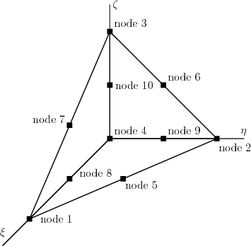
Attribute | Attribute value | Selection of quantities | Used types of selection |
po.dstep = | 0 | – | – |
| number of UDPs npnt | %ld |
|
|
| natural coordinates ξ, η and ζ of UDPs | (%le %le %le)×npnt |
|
| elements | conjugated selection of element ids and UDP ids - see Sect.6.1.1, 6.1.5 and 6.1.6 |
|
| strains, strain transformation, stresses, stress transformation, eqother array | (selection of strain component ids - Sect.6.1.2, strain transfromation flag - {0—-1}, selection of stress component ids - Sect.6.1.2, stress transfromation flag - {0—-1}, selection of eqother array component ids - Sect.6.1.2)×npnt |
In this example, the output of all displacement components will be specified for all nodes.
Example without keywords
| # SELECTION OF REQUIRED NODES | |
| 1 | # type of selection = all nodes |
| # SELECTION OF DISPLACEMENT COMPONENTS | |
| 1 | # type of conjugated selection for all nodes = |
| # = all displacement components selected | |
Example with keywords
| displ_nodes | # SELECTION OF REQUIRED NODES |
| sel_all | # type of selection = all nodes |
| noddispl_comp | # SELECTION OF DISPLACEMENT COMPONENTS |
| sel_all | # type of conjugated selection for all nodes = |
| # = all displacement components selected | |
In this example, the output of all strain components will be specified for nodes 8 and 11. No output of principal strains will be required.
Example without keywords
| # SELECTION OF REQUIRED NODES | |
| 3 | # type of selection = integer list |
| 2 | # two items of list will be specified |
| 8 | # node 8 = item 1. |
| 11 | # node 11 = item 2. |
| # SELECTION OF REQUIRED STRAIN COMPONENTS | |
| 1 | # type of conjugated selection for item 1. = |
| # = all components selected for node 8 | |
| 1 | # type of conjugated selection for item 2. = |
| # = all components selected for node 11 | |
| # FLAGS FOR PRINCIPAL STRESSES | |
| 0 | # item 1. = node 8 -¿ no principal strain |
| 0 | # item 2. = node 11 -¿ no principal strain |
Example with keywords
| strain_nodes | # SELECTION OF REQUIRED NODES |
| sel_list | # type of selection = integer list |
| numlist_items 2 | # two items of list will be specified |
| 8 | # node 8 = item 1. |
| 11 | # node 11 = item 2. |
| nodstrain_comp | # SELECTION OF REQUIRED STRAIN COMPONENTS |
| sel_all | # type of conjugated selection for item 1. = |
| # = all components selected for node 8 | |
| sel_all | # type of conjugated selection for item 2. = |
| # = all components selected for node 11 | |
| nodstre_transfid | # FLAGS FOR PRINCIPAL STRESSES |
| 0 | # 1.item = node 8 -¿ no principal strain |
| 0 | # 2.item = node 11 -¿ no principal strain |
In this example, the output of stress components σx and σz will be specified for nodes 8 and 11. Output of principal stresses will be required at node 11.
Example without keywords
| # SELECTION OF REQUIRED NODES | |
| 3 | # type of selection = integer list |
| 2 | # two items of list will be specified |
| 8 | # node 8 = item 1. |
| 11 | # node 11 = item 2. |
| # SELECTION OF REQUIRED STRESS COMPONENTS | |
| 3 | # type of conjugated selection for item 1. = integer list |
| 2 | # number of selected stress components |
| 1 3 | # indeces of stress vector components |
| 3 | # type of conjugated selection for item 2. = integer list |
| 2 | # number of selected stress components |
| 1 3 | # indeces of stress vector components |
| # FLAGS FOR PRINCIPAL STRESSES | |
| 0 | # item 1. = node 8 -¿ no principal stresses |
| -1 | # item 2. = node 11 -¿ print principal stresses |
Example with keywords
| stress_nodes | # SELECTION OF REQUIRED NODES |
| sel_list | # type of selection = integer list |
| numlist_items 2 | # two items of list will be specified |
| 8 | # node 8 = 1. item |
| 11 | # node 11 = 2. item |
| nodstress_comp | # SELECTION OF REQUIRED STRESS COMPONENTS |
| sel_list | # type of conjugated selection for item 1. |
| numlist_items 2 | # number of selected stress components |
| 1 3 | # ids of stress vector components |
| sel_list | # type of conjugated selection for item 2. |
| numlist_items 2 | # number of selected stress components |
| 1 3 | # ids of stress vector components |
| nodstre_transfid | # FLAGS FOR PRINCIPAL STRESSES |
| 0 | # 1.item = node 8 -¿ no principal stresses |
| -1 | # 2.item = node 11 -¿ print principal stresses |
In this example, the output of plastic strain components εxp, ε yp and ε xyp will be specified for all nodes of the domain calculated.
Example without keywords
| # SELECTION OF REQUIRED NODES | |
| 1 | # type of selection = sel_all |
| # all nodes will be specified | |
| # SELECTION OF PLASTIC STRAIN COMPONENTS | |
| 3 | # type of conjugated selection for all nodes = |
| # = integer list | |
| 3 | # number of selected plastic strain components |
| 1 2 3 | # indeces of eqother array corresponding to |
| # required pl. strain components epsˆp_x and epsˆp_y | |
Example with keywords
| other_nodes | # SELECTION OF REQUIRED NODES |
| sel_all | # type of selection = sel_all |
| # all nodes will be specified | |
| nodother_comp | # SELECTION OF PLASTIC STRAIN COMPONENTS |
| sel_list | # type of conjugated selection for all nodes = |
| # = integer list | |
| numlist_items 3 | # number of selected plastic strain components |
| 1 2 3 | # indeces of eqother array corresponding to |
| # required pl. strain components epsˆp_x and epsˆp_y | |
In this example, the output of all strain components will be specified for integration points of elements 1 and 40-60. Output of principal strains will be required for element 1.
Example without keywords
| # SELECTION OF REQUIRED ELEMENTS | |
| 2 | # type of selection = integer range |
| 2 | # two ranges will be specified |
| # first range <1, 1> | |
| 1 | # initial id - range 1. |
| 1 | # number of selected ids - range 1. |
| # second range <40, 60> | |
| 40 | # initial id - range 2. |
| 20 | # number of selected ids - range 2. |
| # SELECTION OF REQUIRED STRAIN COMPONENTS | |
| 1 | # type of conjugated selection for range 1. = |
| # = all strain components | |
| 1 | # type of conjugated selection for range 2. = |
| # = all strain components | |
| # FLAGS FOR PRINCIPAL STRAINS | |
| -1 | # range 1. -¿ print principal strains |
| 0 | # range 2. -¿ no principal strains |
Example with keywords
| strain_elems | # SELECTION OF REQUIRED ELEMENTS |
| sel_range | # type of selection = integer range |
| num_ranges 2 | # two ranges will be specified |
| # first range <1, 1> | |
| 1 | # initial id - range 1. |
| 1 | # number of selected ids - range 1. |
| # second range <40, 60> | |
| 40 | # initial id - range 2. |
| 20 | # number of selected ids - range 2. |
| elemstrain_comp | # SELECTION OF REQUIRED STRAIN COMPONENTS |
| sel_all | # type of conjugated selection for range 1. = |
| # = all strain components | |
| sel_all | # type of conjugated selection for range 2. = |
| # = all strain components | |
| elemstra_transfid | # FLAGS FOR PRINCIPAL STRAINS |
| -1 | # range 1. -¿ print principal strains |
| 0 | # range 2. -¿ no principal strains |
In this example, the output of all stress components will be specified for integration points of all elements. Output of principal stresses will be required for all elements.
Example without keywords
| # SELECTION OF REQUIRED ELEMENTS | |
| 1 | # type of selection = all ids |
| # SELECTION OF REQUIRED STRESS COMPONENTS | |
| 1 | # type of conjugated selection for all elements = |
| # = all stress components | |
| # FLAGS FOR PRINCIPAL STRAINS | |
| -1 | # print principal stresses for all elements |
Example with keywords
| stress_elems | # SELECTION OF REQUIRED ELEMENTS |
| sel_all | # type of selection = all ids |
| elemstress_comp | # SELECTION OF REQUIRED STRESS COMPONENTS |
| sel_all | # type of conjugated selection for all elements = |
| # = all stress components | |
| # FLAGS FOR PRINCIPAL STRAINS | |
| -1 | # print principal stresses for all elements |
In this example, the output of plastic strain components εxp and ε yp will be specified for integration points of elements 1-25 and 36-40 .
Example without keywords
| # SELECTION OF REQUIRED ELEMENTS | |
| 2 | # type of selection = integer ranges |
| 2 | # two ranges will be specified |
| # first range <1, 25> | |
| 1 | # initial id - range 1. |
| 25 | # number of selected ids - range 1. |
| # second range <36, 40> | |
| 36 | # initial id - range 2. |
| 5 | # number of selected ids - range 2. |
| # SELECTION OF PLASTIC STRAIN COMPONENTS | |
| 3 | # type of conjugated selection for range 1. |
| 2 | # number of selected pl. strain components |
| 1 2 | # indeces of eqother array corresponding to |
| # required pl. strain components epsˆp_x and epsˆp_y | |
| 3 | # type of conjugated selection for range 2. |
| 2 | # number of selected pl. strain components |
| 1 2 | # indeces of eqother array corresponding to |
| # required pl. strain components epsˆp_x and epsˆp_y | |
Example with keywords
| other_elems | # SELECTION OF REQUIRED ELEMENTS |
| sel_range | # type of selection = integer ranges |
| num_ranges 2 | # two ranges will be specified |
| # first range <1, 25> | |
| 1 | # initial id - range 1. |
| 25 | # number of selected ids - range 1. |
| # second range <36, 40> | |
| 36 | # initial id - range 2. |
| 5 | # number of selected ids - range 2. |
| elemother_comp | # SELECTION OF PLASTIC STRAIN COMPONENTS |
| sel_list | # type of conjugated selection for range 1. |
| numlist_items 2 | # number of selected pl. strain components |
| 1 2 | # indeces of eqother array corresponding to |
# required pl. strain components eps _x and eps _x and eps _y _y |
|
| sel_list | # type of conjugated selection for range 2. |
| numlist_items 2 | # number of selected pl. strain components |
| 1 2 | # indeces of eqother array corresponding to |
# required pl. strain components eps _x and eps _x and eps _y _y |
|
After the value of the attribute gf={1,2,3,4} the configuration of the output values for praticular qunatities follows. The graphical output can be configured separately for quantities stored at nodes and integration points on elements. Configuration for nodal quantities is stored in the attribute nog which is instance of the class nodeoutgm. Configuration of output for quantities connected with the integration points on elements is stored in the attribute eog which is instance of the class elemoutgm. Both classes nodeoutgm and elemoutm have attribute dstep type of sel which defines selection of time steps in which the output will be performed. If the dstep is set to the value sel_no then no selection of the quantities follows. Generally, the content of the section configuring the graphical output can be summarized in the following table
In the above table, the name of the graphical output file (attribute outgrfn) can be arbitrary file name which may involve path. The suffix should be chosen with respect to graphical format given by the outdriverm attribute gf. If the gf = 3 = grfmt_gid then the default suffices .res and .msh are appended to the file name specified.
If the gf = 4 = grfmt_gid_sep then the for each quantity is generated separate file name which starts with the given file name (outgrfn) followed by the quantity specifier Additionally, the default suffix .res is appended to the generated file names. The mesh file name is generated in the same way as for the single file format. The following table describes file name generation for the nodal values in the GiD separated file format.
If the stochastic calculation is performed then the generated suffix precedes the simulation number.
| Quantitity | Quantity specifier and suffix |
| appended to the graphical output | |
| file name | |
| nodal displacement | .displ.res |
| nodal strains | .nodal_eps%ld.res |
| (selected by components) | %ld = strain component id |
| nodal principal strains | .nodal_peps%ld.res |
| (selected by components) | %ld = principal strain component id |
| nodal stress | .nodal_sig%ld.res |
| (selected by components) | %ld = stress component id |
| nodal principal stesses | .nodal_psig%ld.res |
| (selected by components) | %ld = principal stress component id |
| nodal other values | .nodal_other%ld.res |
| (selected by components) | %ld = eqother array component id |
| nodal strains | .nodal_eps_v%ld-%ld_s%ld.res |
| (selected as vector) | _v%ld = initial strain component id |
| -%ld = number of vector components | |
| _s%ld = strain selection id | |
| nodal stress | .nodal_sig_v%ld-%ld_s%ld.res |
| (selected as vector) | _v%ld = initial stress component id |
| -%ld = number of vector components | |
| _s%ld = stress selection id | |
| nodal other values | .nodal_other_v%ld-%ld_s%ld.res |
| (selected as vector) | _v%ld = initial eqother component component id |
| -%ld = number of vector components | |
| _s%ld = other value selection id | |
| nodal strains | .nodal_eps_m_s%ld.res |
| (selected as tensor) | _s%ld = strain selection id |
| nodal stress | .nodal_sig_m_s%ld.res |
| (selected as tensor) | _s%ld = stress selection id |
| nodal other values | .nodal_other_m%ld-%ld_s%ld.res |
| (selected as tensor) | _m%ld = initial eqother component component id |
| -%ld = number of tensor components | |
| _s%ld = other value selection id | |
| nodal forces | .force.res |
In the above table, the strain/stress/other selection id represents the order of the conjugated selection of strain/stress/other components. For example, if the nodal stress output configuration described in Section 7.5.2.4 was used for GiD separated format, then the name of the output file for the node 8 would have the suffix .nodal_eps_m_s1.res and for the node 11, the suffix would be .nodal_eps_m_s2.res.
The following table describes file name generation for the values on integration point of elements in the GiD separated file format.
| Quantitity | Quantity specifier and suffix |
| appended to the graphical output | |
| file name | |
| element strains | .elem_eps%ld.res |
| (selected by components) | %ld = strain component id |
| element stresses | .elem_sig%ld.res |
| (selected by components) | %ld = stress component id |
| element other values | .elem_other%ld.res |
| (selected by components) | %ld = eqother array component id |
| element strains | .elem_eps_v%ld-%ld_s%ld.res |
| (selected as vector) | _v%ld = initial strain component id |
| -%ld = number of vector components | |
| _s%ld = strain selection id | |
| element stresses | .elem_sig_v%ld-%ld_s%ld.res |
| (selected as vector) | _v%ld = initial stress component id |
| -%ld = number of vector components | |
| _s%ld = stress selection id | |
| element other values | .elem_other_v%ld-%ld_s%ld.res |
| (selected as vector) | _v%ld = initial eqother component component id |
| -%ld = number of vector components | |
| _s%ld = other value selection id | |
| element strains | .elem_eps_m_s%ld.res |
| (selected as tensor) | _s%ld = strain selection id |
| element stresses | .elem_sig_m_s%ld.res |
| (selected as tensor) | _s%ld = stress selection id |
| element other values | .elem_other_m%ld-%ld_s%ld.res |
| (selected as tensor) | _m%ld = initial eqother component component id |
| -%ld = number of vector components | |
| _s%ld = other value selection id | |
In the above table, the strain/stress/other selection id represents the order of the conjugated selection of strain/stress/other components. For example, if the output configuration of element plastic strain described in Section 7.5.2.9 was used for GiD separated format, then the name of the output file for the first range of elements 1-25 would have the suffix .elem_other_v1-3_s1.res and for the second range of elements 36-40, the suffix would be .elem_other_v1-3_s2.res.
Every configuration of nodal values output in the graphical format can be described by the following table.
Attribute | Attribute value | Selection of quantities | Used types of selection |
nog.dstep = | 0 | – | – |
| 1-6, 10, 11 | load case | see Sect.6.1.2 |
| displacements | conjugated selection of nodal ids and displacement component ids - see Sect.6.1.1,6.1.5 and 7.5.1.4 |
|
|
| strains | conjugated selection of nodal ids, strain component ids and strain transformation flag (see Sect.6.1.1, 6.1.5, 7.5.1.5, 7.5.2.4) |
|
| stresses | conjugated selection of nodal ids, stress component ids and stress transfromation flag (see Sect.6.1.1, 6.1.5, 7.5.1.6 and 7.5.2.5) |
|
| eqother array | conjugated selection of nodal ids and eqother array component ids - see Sect.6.1.1, 6.1.5 and 7.5.1.7 or 7.5.2.6 |
|
| nodal forces | conjugated selection of nodal ids and nodal force component ids - see Sect.6.1.1,6.1.5 and 7.5.2.3 |
The output configuration of element integration point values in the graphical format can be described by the following table.
Attribute | Attribute value | Selection of quantities | Used types of selection |
eog.dstep = | 0 | – | – |
| 1-6, 10, 11 (see | load case | see Sect.6.1.2 |
| strains | conjugated selection of element ids, strain component ids and strain transformation flag (see Sect.6.1.1, 6.1.5, 7.5.1.8) and 7.5.2.7) |
|
|
| stresses | conjugated selection of element ids, stress component ids and stress transfromation flag (see Sect.6.1.1, 6.1.5, 7.5.1.9 and 7.5.2.8) |
|
| eqother array | conjugated selection of nodal ids and eqother array component ids - see Sect.6.1.1, 6.1.5, 7.5.1.10 and 7.5.2.9 |
Should be noted that the output of principal strains and stresses on elements has not been implemented yet and the transformation flags are ignored in this case.
In this example, the output of all nodal force components will be specified for all nodes.
Example without keywords
| # SELECTION OF REQUIRED NODES | |
| 1 | # type of selection = all nodes |
| # SELECTION OF NODAL FORCE COMPONENTS | |
| 1 | # type of conjugated selection for all nodes = |
| # = all nodal force components selected | |
Example with keywords
| force_nodes | # SELECTION OF REQUIRED NODES |
| sel_all | # type of selection = all nodes |
| force_comp | # SELECTION OF NODAL FORCE COMPONENTS |
| sel_all | # type of conjugated selection for all nodes = |
| # = all nodal force components selected | |
In this example, the output of all strain components to GiD in tensorial format will be specified for nodes 8 and 11. No output of principal strains will be required.
Example without keywords
| # SELECTION OF REQUIRED NODES | |
| 3 | # type of selection = integer list |
| 2 | # two items of list will be specified |
| 8 | # node 8 = item 1. |
| 11 | # node 11 = item 2. |
| # SELECTION OF REQUIRED STRAIN COMPONENTS | |
| 7 | # type of conjugated selection for item 1. = |
| # = all components in tensorial format for node 8 | |
| 7 | # type of conjugated selection for item 2. = |
| # = all components in tensorial format for node 11 | |
| # FLAGS FOR PRINCIPAL STRESSES | |
| 0 | # item 1. = node 8 -¿ no principal strain |
| 0 | # item 2. = node 11 -¿ no principal strain |
Example with keywords
| strain_nodes | # SELECTION OF REQUIRED NODES |
| sel_list | # type of selection = integer list |
| numlist_items 2 | # two items of list will be specified |
| 8 | # node 8 = item 1. |
| 11 | # node 11 = item 2. |
| nodstrain_comp | # SELECTION OF REQUIRED STRAIN COMPONENTS |
| sel_mtx | # type of conjugated selection for item 1. = |
| # = all components in tensorial format for node 8 | |
| sel_mtx | # type of conjugated selection for item 2. = |
| # = all components in tensorial format for node 11 | |
| nodstre_transfid | # FLAGS FOR PRINCIPAL STRESSES |
| 0 | # 1.item = node 8 -¿ no principal strain |
| 0 | # 2.item = node 11 -¿ no principal strain |
In this example, the output of all stress components in GiD tensorial format will be specified for all nodes. Output of principal stresses will not be required.
Example without keywords
| # SELECTION OF REQUIRED NODES | |
| 1 | # type of selection = all nodes |
| # SELECTION OF REQUIRED STRESS COMPONENTS | |
| 7 | # type of conjugated selection for all nodes = |
| # = all components in GiD tensorial format | |
| # FLAGS FOR PRINCIPAL STRESSES | |
| -1 | # for all nodes -¿ print principal stresses |
Example with keywords
| stress_nodes | # SELECTION OF REQUIRED NODES |
| sel_all | # type of selection = all nodes |
| nodstress_comp | # SELECTION OF REQUIRED STRESS COMPONENTS |
| sel_mtx | # type of conjugated selection for all nodes = |
| # = all components in GiD tensorial format | |
| nodstre_transfid | # FLAGS FOR PRINCIPAL STRESSES |
| -1 | # for all nodes -¿ print principal stresses |
In this example, the output of plastic strain components εxp, ε yp, ε xyp and ε zp in GiD tensorial format will be specified for all nodes. It is assumed the plain-stress state and therefor only four nonzero components are store in the eqother array.
Example without keywords
| # SELECTION OF REQUIRED NODES | |
| 1 | # type of selection = all nodes |
| # all nodes will be specified | |
| # SELECTION OF PLASTIC STRAIN COMPONENTS | |
| 8 | # type of conjugated selection for all nodes = |
| # = tensorial components selected from large array | |
| 1 | # initial id in eqother array |
| 4 | # number of indeces in eqother array corresponding |
| # to the number of plastic strain components for | |
| # the plane-stress state | |
Example with keywords
| other_nodes | # SELECTION OF REQUIRED NODES |
| sel_all | # type of selection = all nodes |
| # all nodes will be specified | |
| nodother_comp | # SELECTION OF PLASTIC STRAIN COMPONENTS |
| sel_range_mtx | # type of conjugated selection for all nodes = |
| # = tensorial components selected from large array | |
| 1 | # initial id in eqother array |
| 4 | # number of indeces in eqother array corresponding |
| # to the number of plastic strain components for | |
| # the plane-stress state | |
In this example, the output of all strain components in GiD tensorial format will be specified for integration points of elements 40-60 and εx component will be specified for integration point of elements 1-39. Output of principal strains will not be.
Example without keywords
| # SELECTION OF REQUIRED ELEMENTS | |
| 2 | # type of selection = integer range |
| 2 | # two ranges will be specified |
| # first range <1, 39> | |
| 1 | # initial id - range 1. |
| 39 | # number of selected ids - range 1. |
| # second range <40, 60> | |
| 40 | # initial id - range 2. |
| 20 | # number of selected ids - range 2. |
| # SELECTION OF REQUIRED STRAIN COMPONENTS | |
| 3 | # type of conjugated selection for range 1. = |
| # = integer list | |
| 1 | # number of list items |
| 1 | # first component eps_x is selected |
| 7 | # type of conjugated selection for range 2. = |
| # = all strain components in GiD tensorial format | |
| # FLAGS FOR PRINCIPAL STRAINS | |
| -1 | # range 1. -¿ print principal strains |
| 0 | # range 2. -¿ no principal strains |
Example with keywords
| strain_elems | # SELECTION OF REQUIRED ELEMENTS |
| sel_range | # type of selection = integer range |
| num_ranges 2 | # two ranges will be specified |
| # first range <1, 39> | |
| 1 | # initial id - range 1. |
| 39 | # number of selected ids - range 1. |
| # second range <40, 60> | |
| 40 | # initial id - range 2. |
| 20 | # number of selected ids - range 2. |
| elemstrain_comp | # SELECTION OF REQUIRED STRAIN COMPONENTS |
| sel_list | # type of conjugated selection for range 1. = |
| # = integer list | |
| numlist_items 1 | # number of selected items |
| 1 | # the first strain component selected for range 1. |
| sel_mtx | # type of conjugated selection for range 2. = |
| # = all strain components in GiD tensorial format | |
| elemstra_transfid | # FLAGS FOR PRINCIPAL STRAINS |
| 0 | # range 1. -¿ no principal strains |
| 0 | # range 2. -¿ no principal strains |
In this example, the output of all stress components will be specified in GiD tensorial format for integration points of all elements. Output of principal stresses will not be required for all elements.
Example without keywords
| # SELECTION OF REQUIRED ELEMENTS | |
| 1 | # type of selection = all ids |
| # SELECTION OF REQUIRED STRESS COMPONENTS | |
| 7 | # type of conjugated selection for all elements = |
| # = all stress components in GiD tensorial format | |
| # FLAGS FOR PRINCIPAL STRAINS | |
| 0 | # do not print principal stresses for all elements |
Example with keywords
| stress_elems | # SELECTION OF REQUIRED ELEMENTS |
| sel_all | # type of selection = all ids |
| elemstress_comp | # SELECTION OF REQUIRED STRESS COMPONENTS |
| sel_mtx | # type of conjugated selection for all elements = |
| # = all stress components in GiD tensorial format | |
| # FLAGS FOR PRINCIPAL STRAINS | |
| 0 | # do not print principal stresses for all elements |
In this example, the output of plastic strain components εxp, ε yp and ε zp will be specified in GiD vector format for integration points of elements 1-25 and 36-40. The space stress state is assumed in the following examples.
Example without keywords
| # SELECTION OF REQUIRED ELEMENTS | |
| 2 | # type of selection = integer ranges |
| 2 | # two ranges will be specified |
| # first range <1, 25> | |
| 1 | # initial id - range 1. |
| 25 | # number of selected ids - range 1. |
| # second range <36, 40> | |
| 36 | # initial id - range 2. |
| 5 | # number of selected ids - range 2. |
| # SELECTION OF PLASTIC STRAIN COMPONENTS | |
| 9 | # type of conjugated selection for range 1. |
| 1 | # initial id of of epsˆp_x in eqother array |
| 3 | # number of vector components |
| 9 | # type of conjugated selection for range 2. |
| 1 | # initial id of of epsˆp_x in eqother array |
| 3 | # number of vector components |
Example with keywords
| other_elems | # SELECTION OF REQUIRED ELEMENTS |
| sel_range | # type of selection = integer ranges |
| num_ranges 2 | # two ranges will be specified |
| # first range <1, 25> | |
| 1 | # initial id - range 1. |
| 25 | # number of selected ids - range 1. |
| # second range <36, 40> | |
| 36 | # initial id - range 2. |
| 5 | # number of selected ids - range 2. |
| elemother_comp | # SELECTION OF PLASTIC STRAIN COMPONENTS |
| sel_range_vec | # type of conjugated selection for range 1. |
| 1 | # initial id of of epsˆp_x in eqother array |
| 3 | # number of vector components |
| sel_range_vec | # type of conjugated selection for range 2. |
| 1 | # initial id of of epsˆp_x in eqother array |
| 3 | # number of vector components |
The configuration of the tabular output is given by the file name and ndiag times repeated configuration of the particular diagram files.
The file name may be arbitrary including path and suffix. If the number of diagram files is greater than one then the user defined suffix precedes the diagram file number generated automatically. If the stochastic calculation is performed then the user defined suffix including eventual generated diagram file number precedes the simulation number separated by a dot.
Generally, the configuration can be described by the following table.
| Attribute | Description or additional configuration |
| outdiagfn | Output file name (%s) |
| odiag×ndiag | See Table 7.9 |
The attribute odiag is type of class outdiagm which stores the configuration of the diagram file. It contains attribute npun which represents the number of printed unknowns, attribute nif which is array of enumeration nodip (see galias.h) and attribute pu which is array of enumeration prunk (see alias.h). Elements of nif array represents type of points (node/integration point) in which the required unknown will be printed out. Type of points involved in the enumeration nodip are summarized in Table 7.7.
| attribute | enumerator | description |
| nif[i] = 0 | no_point | no point selected |
| nif[i] = 1 | atnode | point is given by node id |
| nif[i] = 2 | atip | point is given by integration point on element |
| nif[i] = 3 | atxyz | point is given by coordinates, |
| the nearest node is selected | ||
Elements of array pu represents types of printed unknown. Type of printed unknowns involved in the enumeration prunk are described in Table 7.8.
| attribute | enumerator | description |
| pu[i] = 1 | pr_displ | print displacement component |
| pu[i] = 2 | pr_strains | print strain component |
| pu[i] = 3 | pr_stresses | print stress component |
| pu[i] = 4 | pr_forces | print nodal force vector component |
| pu[i] = 5 | pr_react | print reaction |
| pu[i] = 6 | pr_stepid | print integer step id |
| pu[i] = 7 | pr_appload | print load coefficient/time of the actual step |
| pu[i] = 8 | pr_other | print eqother array component |
The record for one odiag instance is summarized in Table 7.9.
| Attribute | Description or |
| value | additional configuration |
| odiag.npun | number of printed unknowns (%ld) |
| odiag.dstep = 0 | – |
| odiag.dstep > 0 | npun × (Table 7.10) |
If the attribute dstep of outdiagm class is set to sel_no option then no additional configuration is necessary otherwise the input record for one required unknown is repeated npun times. Description of the input record for one unknown is captured in Table 7.10 and it depeneds on the point type specified. Depending on the point type, the different types of unknowns can be specified - see Table 7.11.
Attribute | Attribute value (see Table 7.7) | Selected point record | Selection of unknown |
odiag.nif[i] = | 0 | – | – |
odiag.nif[i] = | 1 | node id (%ld) | See Table 7.11, |
|
|
| options 1-8 |
odiag.nif[i] = | 2 | element id (%ld) | See Table 7.11, |
|
| local int. point id (%ld) | options 2,3,6-8 |
odiag.nif[i] = | 3 | x coordinate (%le) |
|
|
| y coordinate (%le) | See Table 7.11, |
|
| z coordinate (%le) | options 1-8 |
Attribute | Attribute value | Selected unknown component id |
| (see Table 7.8) |
|
odiag.pu[i] = | 1 | displacement component id (%ld) |
odiag.pu[i] = | 2 | strain component id (%ld) |
odiag.pu[i] = | 3 | stress component id (%ld) |
odiag.pu[i] = | 4 | nodal force component id (%ld) |
odiag.pu[i] = | 5 | reaction component id (%ld) |
odiag.pu[i] = | 6 | – |
odiag.pu[i] = | 7 | – |
odiag.pu[i] = | 8 | eqother array component id (%ld) |
In this example, the J2 flow plasticity material will be assumed. Two table output files will be configured. The first file j2beam.1.dat will contain five columns with step id, horizontal displacement, strain component εy, stress component σx and reaction in vertical direction. The second file j2beam.2.dat will contain two columns with the load coefficient and consistency parameter γ. Each row of the table will contain the value of the given unknown in dependence on all performed time steps either for node 8 or the second integration point of element 12 or the nearest node to point with coordinates [2.3, -5.1, 8.5].
Example without keywords
| 2 | # number of generated table output files |
| j2beam.dat | # basic name of generated the files |
| # the file number will be added automatically | |
| # | |
| # CONFIGURATION OF THE FIRST FILE | |
| 5 | # number of printed unknowns |
| 1 | # type of time step selection = all time steps |
| # 1. column | |
| 1 | # point type = node |
| 8 | # point id = 8. node |
| 6 | # unknown type = step id |
| # 2. column | |
| 3 | # point type = point with coordinates |
| 2.3 -5.1 8.5 | # x, y, z coordinates of point, |
| # the nearset node will be selecetd | |
| 1 | # unknown type = displacement |
| 1 | # component id 1 = horizontal displacement |
| # 3. column | |
| 2 | # point type = integration point |
| 12 2 | # point id = 12. element, 2. int. point |
| 2 | # unknown type = strain |
| 2 | # the second strain component = eps_y |
| # 4. column | |
| 2 | # point type = integration point |
| 12 2 | # point id = 12. element, 2. int. point |
| 3 | # unknown type = stress |
| 1 | # the first stress component = sig_x |
| # 5. column | |
| 1 | # point type = node |
| 8 | # point id = 8. node |
| 5 | # uknown type = reaction |
| 2 | # the second component = vertical reaction |
| # | |
| # CONFIGURATION OF THE SECOND FILE | |
| 2 | # number of printed unknowns |
| 1 | # type of time step selection = all time steps |
| # 1. column | |
| 2 | # point type = integration point |
| 12 2 | # point id = 12. element, 2. int. point |
| 7 | # unknown type = load coefficient |
| # 2. column | |
| 2 | # point type = integration point |
| 12 2 | # point id = 12. element, 2. int. point |
| 8 | # unknown type = eqother array value |
| 5 | # component id 5 = consistency parameter |
Example with keywords
| numdiag 2 | # number of generated table output files |
| j2beam.dat | # basic name of generated the files |
| # the file number will be added automatically | |
| # | |
| # CONFIGURATION OF THE FIRST FILE | |
| numunknowns 5 | # number of printed unknowns |
| sel_all | # type of time step selection = all time steps |
| # 1. column | |
| point atnode | # point type = node |
| node 8 | # point id = 8. node |
| quant_type step_id | # unknown type = step id |
| # 2. column | |
| point atxyz | # point type = point with coordinates |
| x 2.3 y -5.1 z 8.5 | # x, y, z coordinates of point, |
| # the nearset node will be selecetd | |
| quant_type pr_displ | # unknown type = displacement |
| compid 1 | # component id 1 = horizontal displacement |
| # 3. column | |
| point atip | # point type = integration point |
| elem 12 ip 2 | # point id = 12. element, 2. int. point |
| quant_type pr_strain | # unknown type = strain |
| compid 2 | # the second strain component = eps_y |
| # 4. column | |
| point atip | # point type = integration point |
| elem 12 ip 2 | # point id = 12. element, 2. int. point |
| quant_type pr_stress | # unknown type = stress |
| compid 1 | # the first stress component = sig_x |
| # 5. column | |
| point atnode 1 | # point type = node |
| node 8 | # point id = 8. node |
| quant_type pr_react | # uknown type = reaction |
| compid 2 | # the second component = vertical reaction |
| # CONFIGURATION OF THE SECOND FILE | |
| numunknowns 2 | # number of printed unknowns |
| sel_all | # type of time step selection = all time steps |
| # 1. column | |
| point atip | # point type = integration point |
| elem 12 ip 2 | # point id = 12. element, 2. int. point |
| quant_type pr_appload | # unknown type = load coefficient |
| # 2. column | |
| point atip | # point type = integration point |
| elem 12 ip 2 | # point id = 12. element, 2. int. point |
| quant_type pr_other | # unknown type = eqother array value |
| compid 5 | # component id 5 = consistency parameter |
In the following subsections, various types of outdriverm configurations are presented. Their parts can be swapped mutually but the user should be carefull becuase of used material modells and the problem solved. For example in the linear statics problem, the outdiag can be specified but the diagram files are not reasonable in this case because there is no dependence of unknowns on time or load coefficient. Also the output of internal variables stored in the eqother array is not allowed because the linear elastic materials have no internal variables. In such cases, the user should select no elements or nodes for eqother output and zero number of diagram files.
If the output of eqother values such as plastic strains, damage parameters or creep strains is required then the index of variable has to be specified. The order of the internal variables stored in the eqother depeneds on the material model used and it can be found and checked in the source files describing the given model. Usually, the header file should contain description of the appropriate class for material model and the order of the internal varibles should be involved. Definitely, the user can find the order of the internal variables in the member function nlstresses of the given material model.
If the user decides for using of keywords in the outdriver section of the input file for MEFEL then it is necessary to use switch -kwd=2 in the case of no keywords in probdesc section or -kwd=3 in the case of keywords both in probdesc and outdriverm sections.
In this example, the output of all displacements, nodal strains, nodal stresses and reactions will be set to the plain text file and all strains and stresses on elements in tensorial form to the GiD result file. Additionally, nodal displacement will be printed to the GiD result file.
Example without keywords
| # PLAIN TEXT OUTPUT | |
| 1 | # plain text output is produced |
| linstat.out | # file name for the plain text output |
| # Output configuration of nodal values | |
| 1 | # nodal values in all time steps are printed |
| 1 | # nodal values for all load cases are printed |
| 1 | # displacements are printed at all nodes |
| 1 | # all displacement components are printed |
| 1 | # strains are printed at all nodes |
| 1 | # all strain components are printed |
| 0 | # no nodal strain transformation is performed |
| 1 | # stresses are printed at all nodes |
| 1 | # all stress components are printed |
| 0 | # no nodal stress transformation is performed |
| 0 | # no nodes selected =¿ no nodal other value output |
| 1 | # all reactions are printed |
| # Output configuration for elements | |
| 0 | # no time step for elements is selected =¿ |
| # no output on elements | |
| # OUTPUT IN GRAPHICAL FORMATS | |
| 3 | # single GiD file with results is produced |
| linstat | # file name for GiD output (without suffix) |
| # Output configuration of nodal values | |
| 1 | # nodal values in all time steps are printed |
| 1 | # nodal values for all load cases are printed |
| 1 | # displacements are printed at all nodes |
| 1 | # all displacement components are printed |
| 0 | # no node selected =¿ no nodal strain output |
| 0 | # no node selected =¿ no nodal stress output |
| 0 | # no node selected =¿ no nodal other values output |
| 0 | # no node selected =¿ no nodal forces output |
| # Output configuration of element values | |
| 1 | # element values in all time steps are printed |
| 1 | # element values for all load cases are printed |
| 1 | # strains for all elements are printed |
| 7 | # all strain components are printed as tensors |
| 0 | # no strain transformation is performed |
| 1 | # stresses for all elements are printed |
| 7 | # all stress components are printed as tensors |
| 0 | # no stress transformation is performed |
| 0 | # no elements selected =¿ no other values output |
| # OUTPUT OF TABULAR FILE | |
| 0 | # zero number of tabular files =¿ no tabular output |
Example with keywords
| # PLAIN TEXT OUTPUT | ||
| textout | on | # plain text output is produced |
| linstat.out | # file name for the plain text output | |
| # Output configuration of nodal values | ||
| sel_nodstep | sel_all | # nodal values in all time steps are printed |
| sel_nodlc | sel_all | # nodal values for all load cases are printed |
| displ_nodes | sel_all | # displacements are printed at all nodes |
| displ_comp | sel_all | # all displacement components are printed |
| strain_nodes | sel_all | # strains are printed at all nodes |
| nodstrain_comp | sel_all | # all strain components are printed |
| nodstra_transfid | 0 | # no nodal strain transformation is performed |
| stress_nodes | sel_all | # stresses are printed at all nodes |
| nodstress_comp | sel_all | # all stress components are printed |
| nodstre_transfid | 0 | # no nodal stress transformation is performed |
| other_nodes | sel_no | # no nodes selected =¿ no other value output |
| reactions | 1 | # all reactions are printed |
| # Output configuration for elements | ||
| sel_elemstep | sel_no | # no time step for elements is selected =¿ |
| # no output on elements | ||
| # OUTPUT IN GRAPHICAL FORMATS | ||
| outgr_format | grfmt_gid | # single GiD file with results is produced |
| linstat | # file name for GiD output (without suffix) | |
| # Output configuration of nodal values | ||
| sel_nodstep | sel_all | # nodal values in all time steps are printed |
| sel_nodlc | sel_all | # nodal values for all load cases are printed |
| displ_nodes | sel_all | # displacements are printed at all nodes |
| displ_comp | sel_all | # all displacement components are printed |
| strain_nodes | sel_no | # no node selected =¿ no nodal strain output |
| stress_nodes | sel_no | # no node selected =¿ no nodal stress output |
| other_nodes | sel_no | # no node selected =¿ no other values output |
| force_nodes | sel_no | # no node selected =¿ no nodal forces output |
| # Output configuration of element values | ||
| sel_elemstep | sel_all | # element values in all time steps are printed |
| sel_elemlc | sel_all | # element values for all load cases are printed |
| strain_elems | sel_all | # strains for all elements are printed |
| elemstrain_comp | sel_mtx | # all strain components are printed as tensors |
| elemstra_transfid | 0 | # no strain transformation is performed |
| stress_elems | sel_all | # stresses for all elements are printed |
| elemstress_comp | sel_mtx | # all stress components are printed as tensors |
| elemstre_transfid | 0 | # no stress transformation is performed |
| other_elems | 0 | # no elements selected =¿ |
| # no other values output | ||
| # OUTPUT OF TABULAR FILE | ||
| numdiag | 0 | # zero number of tabular files =¿ no tabular output |
In this example, the output of all nodal displacements, element strains, element stresses and element other values will be printed to the plain text file and all strains and stresses at nodes in tensorial form to the GiD result file. Additionally, nodal displacement, damage parameter ω stored in the eqother array and all element stress components will be printed to the GiD result file. The tabular output file will contain required values from the node 9, i.e., horizontal component of displacement in the first column, load coefficent in the second column and the damage parameter ω in the third column.
Example without keywords
| # PLAIN TEXT OUTPUT | |
| 1 | # plain text output is produced |
| scdam.out | # file name for the plain text output |
| # Output configuration of nodal values | |
| 1 | # nodal values in all time steps are printed |
| 1 | # nodal values for all load cases are printed |
| 1 | # displacements are printed at all nodes |
| 1 | # all displacement components are printed |
| 0 | # no node is selected =¿ no strain output |
| 0 | # no node is selected =¿ no stress output |
| 0 | # no node is selected =¿ no other values output |
| 0 | # no reactions are printed |
| # Output configuration for elements | |
| 1 | # element values in all time steps are printed |
| 1 | # element values for all load cases are printed |
| 1 | # strains are printed at all elements |
| 1 | # all strain components are printed |
| 0 | # no element strain transformation is performed |
| 1 | # stresses are printed at all elements |
| 1 | # all stress components are printed |
| 0 | # no element stress transformation is performed |
| 1 | # other values are printed at all elements |
| 1 | # all components of eqother array are printed |
| # OUTPUT IN GRAPHICAL FORMATS | |
| 3 | # single GiD file with results is produced |
| scdam | # file name for GiD output (without suffix) |
| # Output configuration of nodal values | |
| 1 | # nodal values in all time steps are printed |
| 1 | # nodal values for all load cases are printed |
| 1 | # displacements are printed at all nodes |
| 1 | # all displacement components are printed |
| 0 | # no nodes selected =¿ no nodal strain output |
| 0 | # no nodes selected =¿ no nodal stress output |
| 1 | # all nodes selected for other values output |
| 3 | # eqother components are selected by list |
| 1 | # one component is specified in the list |
| 2 | # damage parameter is the second in eqother array |
| 0 | # no node selected =¿ no nodal forces output |
| # Output configuration of element values | |
| 1 | # element values in all time steps are printed |
| 1 | # element values for all load cases are printed |
| 0 | # no elements selected =¿ no strain output |
| 1 | # stresses for all elements are printed |
| 1 | # all stress components are printed as scalars |
| 0 | # no stress transformation is performed |
| 0 | # no elements selected =¿ no other values output |
| # OUTPUT OF TABULAR FILE | |
| 1 | # one tabular file is created |
| scdam.dat | # file name for tabular output |
| 3 | # number of printed unknowns |
| 1 | # values will be printed in all time steps |
| # setup of the first column | |
| 1 | # type of point is node |
| 9 | # node number 9 |
| 1 | # unknown type is displacement |
| 1 | # horizontal component of displacement |
| # setup of the second column | |
| 1 | # type of point is node |
| 9 | # node number 9 |
| 7 | # unknown type = load coefficient |
| # setup of the third column | |
| 1 | # type of point is node |
| 9 | # node number 9 |
| 8 | # unknown type is value from eqother array |
| 2 | # component id 2= damage parameter |
Example with keywords
| # PLAIN TEXT OUTPUT | ||
| textout | on | # plain text output is produced |
| scdam.out | # file name for the plain text output | |
| # Output configuration of nodal values | ||
| sel_nodstep | sel_all | # nodal values in all time steps are printed |
| sel_nodlc | sel_all | # nodal values for all load cases are printed |
| displ_nodes | sel_all | # displacements are printed at all nodes |
| displ_comp | sel_all | # all displacement components are printed |
| strain_nodes | sel_no | # no nodes selected =¿ no strain output |
| stress_nodes | sel_no | # no nodes selected =¿ no stress output |
| other_nodes | sel_no | # no nodes selected =¿ no other value output |
| reactions | 0 | # no reactions are printed |
| # Output configuration for elements | ||
| sel_elemstep | sel_all | # element values in all time steps are printed |
| sel_elemlc | sel_all | # element values for all load cases are printed |
| strain_elems | sel_all | # strains for all elements are printed |
| elemstrain_comp | sel_all | # all strain components are printed as tensors |
| elemstra_transfid | 0 | # no strain transformation is performed |
| stress_elems | sel_all | # stresses for all elements are printed |
| elemstress_comp | sel_all | # all stress components are printed |
| other_elems | sel_all | # no elements are selected =¿ no other values output |
| elemoth_comp | sel_all | # all eqother components are printed |
| # OUTPUT IN GRAPHICAL FORMATS | ||
| outgr_format | grfmt_gid | # single GiD file with results is produced |
| scdam | # file name for GiD output (without suffix) | |
| # Output configuration of nodal values | ||
| sel_nodstep | sel_all | # nodal values in all time steps are printed |
| sel_nodlc | sel_all | # nodal values for all load cases are printed |
| displ_nodes | sel_all | # displacements are printed at all nodes |
| displ_comp | sel_all | # all displacement components are printed |
| strain_nodes | sel_no | # no node selected =¿ no nodal strain output |
| stress_nodes | sel_no | # no node selected =¿ no nodal stress output |
| other_nodes | sel_no | # all nodes selected for other values output |
| nodoth_comp | sel_list | # eqother components are selected by list of ids |
| 1 | # one component is specified in the list | |
| 2 | # damage parameter is the second in eqother array | |
| force_nodes | sel_no | # no node selected =¿ no nodal forces output |
| # Output configuration of element values | ||
| sel_elemstep | sel_all | # element values in all time steps are printed |
| sel_elemlc | sel_all | # element values for all load cases are printed |
| strain_elems | sel_no | # no element selected =¿ no strain output |
| stress_elems | sel_all | # stresses for all elements are printed |
| elemstress_comp | sel_all | # all stress components are printed as scalars |
| elemstre_transfid | 0 | # no stress transformation is performed |
| other_elems | 0 | # no elements are selected =¿ no other values output |
| # OUTPUT OF TABULAR FILES | ||
| numdiag | 1 | # one tabular file is created |
| scdam.dat | # file name for tabular output | |
| numunknowns | 3 | # number of printed unknowns |
| 1 | # values will be printed in all time steps | |
| # setup of the first column | ||
| point | atnode | # type of point is node |
| node | 9 | # node number 9 |
| quant_type | pr_displ | # unknown type is displacement |
| compid | 1 | # horizontal component of displacement |
| # setup of the second column | ||
| point | atnode | # type of point is node |
| node | 9 | # node number 9 |
| quant_type | pr_appload | # unknown type = load coefficient |
| # setup of the third column | ||
| point | atnode | # type of point is node |
| node | 9 | # node number 9 |
| quant_type | pr_other | # unknown type = eqother array value |
| compid | 2 | # component id 2= damage parameter |
Type of tansport analysis is stored in the attribute tprob of the class probdesct. The appropriate keyword is problemtype. Values of the attribute tprob are summarized in Table 8.1.
| attribute | enumerator | description |
| tprob = 50 | stationary_problem | linear stationary problem |
| tprob = 51 | nonlinear_stationary_problem | non-linear stationary problem |
| tprob = 60 | nonstationary_problem | non-stationary problem |
| tprob = 61 | nonlinear_nonstationary_problem | non-linear non-stationary problem |
| tprob = 62 | discont_nonstat_problem | discontinuous non-stationary problem |
| tprob = 63 | discont_nonlin_nonstat_problem | discontinuous non-linear |
| non-stationary problem | ||
| tprob = 70 | growing_np_problem | non-stationary problem with |
| changing number of nodes | ||
Array name contains name or description of problem solved. The name is defined by user.
The attribute Mesprt describes the detailness of the auxiliary prints on screen. The appropriate keyword is mesprt.
| attribute | description |
| Mesprt = 0 | no auxiliary print on screen |
| Mesprt = 1 | auxiliary print on screen |
The attribute tmatt describes the type of transport. The keyword is transmatter. Values of the attribute tmatt are summarized in Table 8.3.
| attribute | enumerator | description |
| tmatt = 0 | nomedium | no transport |
| tmatt = 1 | onemedium | transport of a single material/medium |
| tmatt = 10 | twomediacoup | coupled transport of two media |
| tmatt = 30 | threemediacoup | coupled transport of three media |
| tmatt = 40 | fourmediacoup | coupled transport of four media |
The attribute mednam describes the type of transport. The keyword is mednames. Values of the attribute mednam are summarized in Table 8.4.
| attribute | enumerator | description |
| mednam = 1 | heat | heat transport |
| mednam = 2 | moisture | transport of moisture |
| mednam = 10 | heat_moisture | coupled heat and moisture transport |
| mednam = 20 | moisture_salt | coupled salt and moisture transport |
The attributes scale1, scale2, scale3 and scale4 with the keywords scale1, scale2, scale3 and scale4 are used for scaling of all quantities conected with the appropriate medium. These attributes are usually equal to 1.
The attribute tgravity with the keyword gravityacceleration describes whether the gravity acceleration is taken into account. The values of the attribute tgravity is summarized in Table 8.5.
| attribute | enumerator | description |
| tgravity = 0 | gr_no | the gravity acceleration is not taken into account |
| tgravity = 1 | gr_yes | the gravity acceleration is taken into account |
The attribute adaptivityflag describes whether the adaptivity is applied. The appropriate keyword is adaptivity.
| attribute | description |
| adaptivityflag = 0 | adaptivity is not applied (default value) |
| adaptivityflag = 1 | adaptivity is applied (not described now) |
The attribute stochasticcalc describes the type of analysis with respect to deterministic or non-deterministic feature. The appropriate keyword is stochasticcalc.
| attribute | description |
| stochasticcalc = 0 | deterministic approach/computation (default value) |
| stochasticcalc = 1 | stochastic/fuzzy computation, data are read all at once |
| stochasticcalc = 2 | stochastic/fuzzy computation, data are read sequentially |
| stochasticcalc = 3 | stochastic/fuzzy computation, data are generated in the code |
The attribute homogt describes whether homogenization is applied. The appropriate keyword is homogenization.
| attribute | description |
| homogt = 0 | homogenization is not applied (default value) |
| homogt = 1 | homogenization is applied on a single processor |
| homogt = 2 | homogenization is applied on a parallel computer |
Storage of the conductivity matrix is located in the attribute tstorkm of the class probdesct. The appropriate keyword is conductmatstor. Storage of the capacity matrix is located in the attribute tstorcm of the class probdesct. The appropriate keyword is capacmatstor.
The attribute tprt with the keyword timetypeprint describes time units used in output.
| attribute | enumerator | description |
| tprt = 1 | secondst | output in seconds |
| tprt = 2 | minutest | output in minutes |
| tprt = 3 | hourst | output in hours |
| tprt = 4 | dayst | output in days |
The attribute diagcap with the keyword diagonalization determines whether the capacity matrix is diagonalized.
| attribute | description |
| diagcap = 0 | the capacity matrix is not diagonalized |
| diagcap = 1 | the capacity matrix is diagonalized |
Every linear stationary problem is described by the following scheme.
| name of problem solved by user | |
| message printing | Table 8.2 |
| tprob = stationary_problem = 50 | Table 7.1 |
| type of transport | Table 8.3 |
| medium names | Table 8.4 |
| scales | default value i s1 |
| gradients computation | described in Section 2.10 |
| fluxes computation | described in Section 2.11 |
| internal variables computation | described in Section 2.9 |
| internal variables computation | described in Section 2.9 |
| gravity acceleration | Table 8.5 |
| adaptivity | Table 8.6 |
| deterministic/stochastic computation | Table 8.7 |
| homogenization | Table 8.8 |
| node renumbering | described in Section 2.6 |
| storage of the conductivity matrix | described in Section 2.2 |
| solver of linear equations | described in Section 2.3 |
Example without keywords
heat transfer | |
| 1 | # message printing |
| 50 | # linear stationary problem |
| 1 | # type of transport - one medium |
| 1 | # name of the medium - heat |
| 1.0 | # scale |
| 1 | # gradients are computed and stored |
| 2 | # gradients computed in nodes |
| 1 | # the final gradients are average values of gradients from adjacent elements |
| 1 | # fluxes are computed and stored |
| 2 | # fluxes are computed in nodes |
| 1 | # the final fluxes are average values of fluxes from adjacent elements |
| 0 | # internal variables are not computed |
| 0 | # internal variables are not computed |
| 0 | # the gravity is not taken into account |
| 0 | # adaptivity is not applied |
| 0 | # deterministic computation |
| 0 | # homogenization is not used |
| 0 | # no node renumbering |
| 2 | # the conductivity matrix is stored in skyline storage scheme |
| 2 | # system of linear equations is solved by the LDLT factorization |
Example with keywords
heat transfer | |
| mesprt 1 | # message printing |
| problemtype stationary_problem | # linear stationary problem |
| transmatter nomedium | # type of transport - one medium |
| mednames heat | # name of the medium - heat |
| scale1 1.0 | # scale |
| gradcomp 1 | # gradients are computed and stored |
| gradpos 2 | # gradients computed in nodes |
| gradaver 1 | # the final gradients are average values of gradients from adjacent elements |
| fluxcomp 1 | # fluxes are computed and stored |
| fluxpos 2 | # fluxes are computed in nodes |
| fluxaver 1 | # the final fluxes are average values of fluxes from adjacent elements |
| othercomp 0 | # internal variables are not computed |
| eqothercomp 0 | # internal variables are not computed |
| gravityacceleration gr_no | # the gravity is not taken into account |
| adaptivity 0 | # adaptivity is not applied |
| stochasticcalc 0 | # deterministic computation |
| homogenization 0 | # homogenization is not used |
| noderenumber no_renumbering | # no node renumbering |
| conductmatstor skyline_matrix | # the conductivity matrix is stored in skyline storage scheme |
| typelinsol ldl | # system of linear equations is solved by the LDLT factorization |
Every linear non-stationary problem is described by the following scheme.
| name of problem solved by user | |
| message printing | Table 8.2 |
| tprob = nonstationary_problem = 60 | Table 7.1 |
| type of transport | Table 8.3 |
| medium names | Table 8.4 |
| scales | default value i s1 |
| gradients computation | described in Section 2.10 |
| fluxes computation | described in Section 2.11 |
| internal variables computation | described in Section 2.9 |
| internal variables computation | described in Section 2.9 |
| gravity acceleration | Table 8.5 |
| adaptivity | Table 7.4 |
| deterministic/stochastic computation | Table 7.5 |
| homogenization | Table 8.8 |
| node renumbering | described in Section 2.6 |
| time controller | described in Section 2.5 |
| time print | Table 8.9 |
| back-up | |
| parameter of the generalized trapezoidal rule | |
| storage of the conductivity matrix | described in Section 2.2 |
| storage of the capacity matrix | described in Section 2.2 |
| solver of linear equations | described in Section 2.3 |
| diagonalization of the capacity matrix | Table 8.10 |
Example without keywords
heat transfer | |
| 1 | # message printing |
| 60 | # linear non-stationary problem |
| 1 | # type of transport - one medium |
| 1 | # name of the medium - heat |
| 1.0 | # scale |
| 1 | # gradients are computed and stored |
| 2 | # gradients computed in nodes |
| 1 | # the final gradients are average values of gradients from adjacent elements |
| 1 | # fluxes are computed and stored |
| 2 | # fluxes are computed in nodes |
| 1 | # the final fluxes are average values of fluxes from adjacent elements |
| 0 | # internal variables are not computed |
| 0 | # internal variables are not computed |
| 0 | # the gravity is not taken into account |
| 0 | # adaptivity is not applied |
| 0 | # deterministic computation |
| 0 | # homogenization is not used |
| 0 | # no node renumbering |
| 0 | # the type of time controller - fixed |
| 0.0 | # the starting time |
| 123.0 | # the end time |
| 0 | # the number of important times |
| 0 | # the type of general function governing the time step |
| # the constant value | |
| 2.5 | # the time step |
| 1 | # time units in output are seconds |
| 0 | # no back-up (default value) |
| 0.5 | # parameter alpha in the generalized trapezoidal method |
| 2 | # the conductivity matrix is stored in skyline storage scheme |
| 2 | # the capacity matrix is stored in skyline storage scheme |
| 2 | # system of linear equations is solved by the LDLT factorization |
| 0 | # the capacity matrix is not diagonalized |
Example with keywords
heat transfer | |
| mesprt 1 | # message printing |
| problemtype nonstationary_problem | # linear non-stationary problem |
| transmatter onemedium | # type of transport - one medium |
| mednames heat | # name of the medium - heat |
| scale1 1.0 | # scale |
| gradcomp 1 | # gradients are computed and stored |
| gradpos 2 | # gradients computed in nodes |
| gradaver 1 | # the final gradients are average values of gradients from adjacent elements |
| fluxcomp 1 | # fluxes are computed and stored |
| fluxpos 2 | # fluxes are computed in nodes |
| fluxaver 1 | # the final fluxes are average values of fluxes from adjacent elements |
| othercomp 0 | # internal variables are not computed |
| eqothercomp 0 | # internal variables are not computed |
| gravityacceleration gr_no | # the gravity is not taken into account |
| adaptivity 0 | # adaptivity is not applied |
| stochasticcalc 0 | # deterministic computation |
| homogenization 0 | # homogenization is not used |
| noderenumber no_renumbering | # no node renumbering |
| time_contr_type fixed | # the type of time controller - fixed |
| 0.0 | # the starting time |
| 123.0 | # the end time |
| 0 | # the number of important times |
| funct_type stat | # the type of general function - the constant value |
| const_val 2.5 | # the time step |
| timetypeprint secondst | # time units in output are seconds |
| hdbackup nohdb | # no back-up (default value) |
| alpha_integration 0.5 | # parameter alpha in the generalized trapezoidal method |
| conductmatstor skyline_matrix | # the conductivity matrix is stored in skyline storage scheme |
| capacmatstor skyline_matrix | # the capacity matrix is stored in skyline storage scheme |
| typelinsol ldl | # system of linear equations is solved by the LDLT factorization |
| diagcap 0 | # the capacity matrix is not diagonalized |